Exam 13: Consumption and the Aggregate Expenditures Model

Consider a simple aggregate expenditure model where all components of aggregate expenditure are autonomous except consumption. The marginal propensity to consume is 0.75. Suppose the equilibrium level of real GDP at the prevailing price is $600 billion below potential real GDP. All else constant, by how much should autonomous aggregate expenditures be increased to reach potential output?

According to the interest-rate effect, higher prices

Holding all else constant, a change in autonomous aggregate expenditures will shift in aggregate demand by an amount equal to

Consider a simple aggregate expenditure model where all components of aggregate expenditure are autonomous except consumption. Which of the following events causes the aggregate expenditures curve to shift downwards?

An increase in wealth is likely to shift the consumption function curve upward.

Consider a simple aggregate expenditure model where all components of aggregate expenditure are autonomous except consumption. If the consumption function is JC = $500 + 0.8Y, planned investment = $200, government purchases = $300, Jnet exports = $100, and real GDP = $1,000, what is the amount of autonomous expenditures?

In the aggregate expenditures model, in equilibrium,

What is the difference between the aggregate expenditures curve and the aggregate demand Jcurve?

An increase in autonomous aggregate expenditures

According to the real wealth effect, if you are living in a period of rising price levels, the cost of the goods and services you buy

Aggregate expenditures that do not vary with real GDP are called autonomous aggregate Jexpenditures.

Consider a simple aggregate expenditure model where all components of aggregate expenditure are autonomous except consumption. If government purchases increases by $200 billion, the aggregate expenditures curve will shift up by

Let Y = real GDP and Y_d = disposable income. Suppose initially, Y = Y_d and the marginal propensity to consume (MPC) is 0.8. All components of aggregate expenditures except consumption are autonomous. Now suppose the government imposes an income tax rate of 30% on real GDP. As a result, one additional dollar will increase consumption by

What is the multiplier effect, that is, why does income change by a multiple of the initial Jchange in autonomous aggregate expenditures?

The aggregate demand traces

Consider a simple aggregate expenditure model where all components of aggregate expenditure are autonomous except consumption. The marginal propensity to consume is 0.8. Suppose the equilibrium level of real GDP at the prevailing price is $500 billion below potential real GDP. All else constant, by how much should autonomous aggregate expenditures be increased to reach potential output?

Difficulty: Medium Figure 13-4 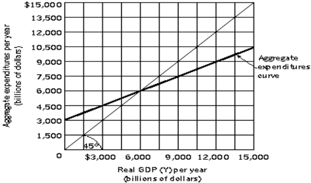-Refer to Figure 13-4. Let Y = real GDP, AE = Aggregate Expenditures, C = Consumption, JI_P = Planned Investment. Suppose AE = C + I_P. I_P is autonomous and the consumption function is C = $1,000 billion + 0.5Y. If real GDP = $7,000 billion, what is the amount of aggregate expenditures?

Difficulty: Medium Figure 13-4 -Refer to Figure 13-4. Let Y = real GDP, AE = Aggregate Expenditures, C = Consumption, JI_P = Planned Investment. Suppose AE = C + I_P, and I_P is autonomous. If the level of real GDP equals $7,000 billion, and if there are no changes in the consumption function or in planned investment, then we expect that, in the next period, real GDP will

Figure 13-5 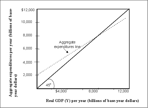-Refer to Figure 13-5. Let Y = real GDP, AE = Aggregate Expenditures, C = Consumption, JI_P = Planned Investment and Y* = equilibrium real GDP. Suppose AE = C + I_P, I_P is autonomous and the consumption function is C = $1,000 billion + 0.75Y. If firms produced a real GDP less than the Y*,

Disposable personal income is