Exam 16: Multiple Regression Model Building

In data mining where huge data sets are being explored to discover relationships among a large number of variables,the best-subsets approach is more practical than the stepwise regression approach.

Instruction 16-6 Given below are results from the regression analysis on 40 observations where the dependent variable is the number of weeks a worker is unemployed due to a layoff (Y) and the independent variables are the age of the worker (X₁), the number of years of education received (X₂), the number of years at the previous job (X₃), a dummy variable for marital status (X₄: 1 = married, 0 = otherwise), a dummy variable for head of household (X₅: 1 = yes, 0 = no) and a dummy variable for management position (X₆: 1 = yes, 0 = no). The coefficient of multiple determination (R²_j) the regression model using each of the 6 variables X_j as the dependent variable and all other X variables as independent variables are, respectively, 0.2628, 0.1240, 0.2404, 0.3510, 0.3342 and 0.0993. The partial results from best-subset regression are given below: Model R Square Adj. R Square Std. Error 0.4568 0.4116 18.3534 0.4697 0.4091 18.3919 0.4691 0.4084 18.4023 0.4877 0.4123 18.3416 0.4949 0.4030 18.4861 -Referring to Instruction 16-6,the model that includes X₁,X₂,X₃,X₅ and X₆ should be among the appropriate models using the Mallow's C_p statistic.

If a group of independent variables are not significant individually but are significant as a group at a specified level of significance,this is most likely due to

Instruction 16-2 A chemist employed by a pharmaceutical firm has developed a muscle relaxant. She took a sample of 14 people suffering from extreme muscle constriction. She gave each a vial containing a dose (X) of the drug and recorded the time to relief (Y) measured in seconds for each. She fit a quadratic model to this data. The results obtained by Microsoft Excel follow. OUTPU? Regression Statistics Multiple R 0.747 R Square 0.558 Adj. R Square 0.478 Std. Error 863.1 Observations 14 ANOVA df Ss MS F Signif F Regression 2 10,344,797 5,172,399 6.94 0.0110 Residual 11 8,193,929 744,903 Total 13 18,538,726 Coeff Std. Error t stat P -value Intercept 1283.0 352.0 3.65 0.0040 CenDose 25.228 8.631 2.92 0.0140 CenDoseSq 0.8604 0.3722 2.31 0.0410 Note: Adj. R Square = Adjusted R Square; Std. Error = Standard Error -Referring to Instruction 16-2,suppose the chemist decides to use a t test to determine if the linear term is significant.Using a level of significance of 0.05,she would decide that the quadratic model should include a linear term.

A regression diagnostic tool used to study the possible effects of collinearity is

Instruction 16-6 Given below are results from the regression analysis on 40 observations where the dependent variable is the number of weeks a worker is unemployed due to a layoff (Y) and the independent variables are the age of the worker (X₁), the number of years of education received (X₂), the number of years at the previous job (X₃), a dummy variable for marital status (X₄: 1 = married, 0 = otherwise), a dummy variable for head of household (X₅: 1 = yes, 0 = no) and a dummy variable for management position (X₆: 1 = yes, 0 = no). The coefficient of multiple determination (R²_j) the regression model using each of the 6 variables X_j as the dependent variable and all other X variables as independent variables are, respectively, 0.2628, 0.1240, 0.2404, 0.3510, 0.3342 and 0.0993. The partial results from best-subset regression are given below: Model R Square Adj. R Square Std. Error 0.4568 0.4116 18.3534 0.4697 0.4091 18.3919 0.4691 0.4084 18.4023 0.4877 0.4123 18.3416 0.4949 0.4030 18.4861 -Referring to Instruction 16-6,there is reason to suspect collinearity between some pairs of predictors based on the values of the variance inflationary factor.

Instruction 16-6 Given below are results from the regression analysis on 40 observations where the dependent variable is the number of weeks a worker is unemployed due to a layoff (Y) and the independent variables are the age of the worker (X₁), the number of years of education received (X₂), the number of years at the previous job (X₃), a dummy variable for marital status (X₄: 1 = married, 0 = otherwise), a dummy variable for head of household (X₅: 1 = yes, 0 = no) and a dummy variable for management position (X₆: 1 = yes, 0 = no). The coefficient of multiple determination (R²_j) the regression model using each of the 6 variables X_j as the dependent variable and all other X variables as independent variables are, respectively, 0.2628, 0.1240, 0.2404, 0.3510, 0.3342 and 0.0993. The partial results from best-subset regression are given below: Model R Square Adj. R Square Std. Error 0.4568 0.4116 18.3534 0.4697 0.4091 18.3919 0.4691 0.4084 18.4023 0.4877 0.4123 18.3416 0.4949 0.4030 18.4861 -Referring to Instruction 16-6,the variable X₄ should be dropped to remove collinearity.

Instruction 16-6 Given below are results from the regression analysis on 40 observations where the dependent variable is the number of weeks a worker is unemployed due to a layoff (Y) and the independent variables are the age of the worker (X₁), the number of years of education received (X₂), the number of years at the previous job (X₃), a dummy variable for marital status (X₄: 1 = married, 0 = otherwise), a dummy variable for head of household (X₅: 1 = yes, 0 = no) and a dummy variable for management position (X₆: 1 = yes, 0 = no). The coefficient of multiple determination (R²_j) the regression model using each of the 6 variables X_j as the dependent variable and all other X variables as independent variables are, respectively, 0.2628, 0.1240, 0.2404, 0.3510, 0.3342 and 0.0993. The partial results from best-subset regression are given below: Model R Square Adj. R Square Std. Error 0.4568 0.4116 18.3534 0.4697 0.4091 18.3919 0.4691 0.4084 18.4023 0.4877 0.4123 18.3416 0.4949 0.4030 18.4861 -Referring to Instruction 16-6,the model that includes all six independent variables should be selected using the adjusted r² statistic.

Instruction 16-6 Given below are results from the regression analysis on 40 observations where the dependent variable is the number of weeks a worker is unemployed due to a layoff (Y) and the independent variables are the age of the worker (X₁), the number of years of education received (X₂), the number of years at the previous job (X₃), a dummy variable for marital status (X₄: 1 = married, 0 = otherwise), a dummy variable for head of household (X₅: 1 = yes, 0 = no) and a dummy variable for management position (X₆: 1 = yes, 0 = no). The coefficient of multiple determination (R²_j) the regression model using each of the 6 variables X_j as the dependent variable and all other X variables as independent variables are, respectively, 0.2628, 0.1240, 0.2404, 0.3510, 0.3342 and 0.0993. The partial results from best-subset regression are given below: Model R Square Adj. R Square Std. Error 0.4568 0.4116 18.3534 0.4697 0.4091 18.3919 0.4691 0.4084 18.4023 0.4877 0.4123 18.3416 0.4949 0.4030 18.4861 -Referring to Instruction 16-6,the variable X₅ should be dropped to remove collinearity.

Instruction 16-6 Given below are results from the regression analysis on 40 observations where the dependent variable is the number of weeks a worker is unemployed due to a layoff (Y) and the independent variables are the age of the worker (X₁), the number of years of education received (X₂), the number of years at the previous job (X₃), a dummy variable for marital status (X₄: 1 = married, 0 = otherwise), a dummy variable for head of household (X₅: 1 = yes, 0 = no) and a dummy variable for management position (X₆: 1 = yes, 0 = no). The coefficient of multiple determination (R²_j) the regression model using each of the 6 variables X_j as the dependent variable and all other X variables as independent variables are, respectively, 0.2628, 0.1240, 0.2404, 0.3510, 0.3342 and 0.0993. The partial results from best-subset regression are given below: Model R Square Adj. R Square Std. Error 0.4568 0.4116 18.3534 0.4697 0.4091 18.3919 0.4691 0.4084 18.4023 0.4877 0.4123 18.3416 0.4949 0.4030 18.4861 -Referring to Instruction 16-6,the model that includes X₁,X₃,X₅ and X₆ should be among the appropriate models using the Mallow's C_p statistic.

Instruction 16-6 Given below are results from the regression analysis on 40 observations where the dependent variable is the number of weeks a worker is unemployed due to a layoff (Y) and the independent variables are the age of the worker (X₁), the number of years of education received (X₂), the number of years at the previous job (X₃), a dummy variable for marital status (X₄: 1 = married, 0 = otherwise), a dummy variable for head of household (X₅: 1 = yes, 0 = no) and a dummy variable for management position (X₆: 1 = yes, 0 = no). The coefficient of multiple determination (R²_j) the regression model using each of the 6 variables X_j as the dependent variable and all other X variables as independent variables are, respectively, 0.2628, 0.1240, 0.2404, 0.3510, 0.3342 and 0.0993. The partial results from best-subset regression are given below: Model R Square Adj. R Square Std. Error 0.4568 0.4116 18.3534 0.4697 0.4091 18.3919 0.4691 0.4084 18.4023 0.4877 0.4123 18.3416 0.4949 0.4030 18.4861 -Referring to Instruction 16-6,what is the value of the variance inflationary factor of Edu?

Which of the following is used to find a 'best' model?

Instruction 16-6 Given below are results from the regression analysis on 40 observations where the dependent variable is the number of weeks a worker is unemployed due to a layoff (Y) and the independent variables are the age of the worker (X₁), the number of years of education received (X₂), the number of years at the previous job (X₃), a dummy variable for marital status (X₄: 1 = married, 0 = otherwise), a dummy variable for head of household (X₅: 1 = yes, 0 = no) and a dummy variable for management position (X₆: 1 = yes, 0 = no). The coefficient of multiple determination (R²_j) the regression model using each of the 6 variables X_j as the dependent variable and all other X variables as independent variables are, respectively, 0.2628, 0.1240, 0.2404, 0.3510, 0.3342 and 0.0993. The partial results from best-subset regression are given below: Model R Square Adj. R Square Std. Error 0.4568 0.4116 18.3534 0.4697 0.4091 18.3919 0.4691 0.4084 18.4023 0.4877 0.4123 18.3416 0.4949 0.4030 18.4861 -Referring to Instruction 16-6,the model that includes X₁,X₂,X₅ and X₆ should be among the appropriate models using the Mallow's C_p statistic.

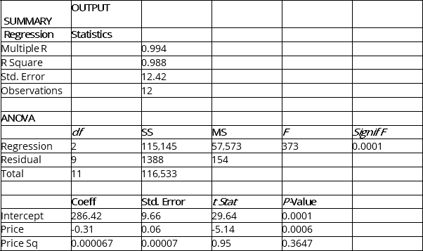
Instruction 16-4 A certain type of rare gem serves as a status symbol for many of its owners. In theory, for low prices, the demand decreases as the price of the gem increases. However, experts hypothesise that when the gem is valued at very high prices, the demand increases with price due to the status owners believe they gain in obtaining the gem. Thus, the model proposed to best explain the demand for the gem by its price is the quadratic model: Y = β₀ + β₁X + β₂X² + ^ε where Y = demand (in thousands) and X = retail price per carat. This model was fit to data collected for a sample of 12 rare gems of this type. A portion of the computer analysis obtained from Microsoft Excel is shown below: Note: Std. Error = Standard Error -Referring to Instruction 16-4,and noting that this model includes both a linear and a quadratic term,what is the correct interpretation of the coefficient of multiple determination?

In multiple regression,the_______ procedure permits variables to enter and leave the model at different stages of its development.

A regression diagnostic tool used to study the possible effects of collinearity is _______.

Unethical behaviour occurs when someone uses multiple regression analysis and wilfully fails to remove from consideration variables that exhibit a high collinearity with other independent variables.

Instruction 16-6 Given below are results from the regression analysis on 40 observations where the dependent variable is the number of weeks a worker is unemployed due to a layoff (Y) and the independent variables are the age of the worker (X₁), the number of years of education received (X₂), the number of years at the previous job (X₃), a dummy variable for marital status (X₄: 1 = married, 0 = otherwise), a dummy variable for head of household (X₅: 1 = yes, 0 = no) and a dummy variable for management position (X₆: 1 = yes, 0 = no). The coefficient of multiple determination (R²_j) the regression model using each of the 6 variables X_j as the dependent variable and all other X variables as independent variables are, respectively, 0.2628, 0.1240, 0.2404, 0.3510, 0.3342 and 0.0993. The partial results from best-subset regression are given below: Model R Square Adj. R Square Std. Error 0.4568 0.4116 18.3534 0.4697 0.4091 18.3919 0.4691 0.4084 18.4023 0.4877 0.4123 18.3416 0.4949 0.4030 18.4861 -Referring to Instruction 16-6,the model that includes X₁,X₅ and X₆ should be among the appropriate models using the Mallow's C_p statistic.

Using the best-subsets approach to model building,models are being considered when their

A certain type of rare gem serves as a status symbol for many of its owners. In theory, for low prices, the demand decreases as the price of the gem increases. However, experts hypothesise that when the gem is valued at very high prices, the demand increases with price due to the status owners believe they gain in obtaining the gem. Thus, the model proposed to best explain the demand for the gem by its price is the quadratic model: $Y = B _ { 0 } + B _ { 1 } X + B_ { 2 } X ^ { 2 } + \varepsilon$ where Y = demand (in thousands) and X = retail price per carat. SUMMARY OUTPUT Regression Statistics Multiple R 0.994 R Square 0.988 Std. Error 12.42 Observations 12 ANOVA df SS MS F Signif F Regression 2 115,145 57,573 373 0.0001 Residual 9 1,388 154 Total 11 116,533 Coeff Std. Error t Stat P -Value Intercept 286.42 9.66 29.64 0.0001 Price -0.31 0.06 -5.14 0.0006 Price Sq 0.000067 0.00007 0.95 0.3647 This model was fit to data collected for a sample of 12 rare gems of this type. A portion of the computer analysis obtained from Microsoft Excel is shown below: -Referring to Instruction 16-1,what is the p-value associated with the test statistic for testing whether the quadratic term is necessary in fitting the response curve relating the demand (Y)and the price (X)?