Exam 15: Random- and Mixed-Effects Analysis of Variance Models

Correct Answer:

Verified

Procedure:
Create a data set with three variables: Time 1, Time 2, and Time 3. The data set should have 12 cases, representing 12 teachers.

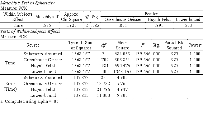
1. Go to Analyze $\rightarrow$ General Linear Model $\rightarrow$ Repeated Measures.
"2. For Within-Subject Factor Name, enter ""Time.""
For Number of Levels, enter 3 (i.e., 3 time points). Click Add.
For Measure Name, enter ""PCK."" Click Add."
3. Click Define. Move Time1 through Time3 in the left box to Within-Subjects Variables (Time).
4. Click Options. Move "Time" to Display Means for. Select Compare main effects. Select Bonferroni under Confidence interval adjustment. Select Descriptive statistics, Estimates of effect size, and Observed power. Click Continue.
5. To get profile plots, click Plots. Move "Time" to the box under Horizontal Axis. Click Add. Click Continue.
"6. Click OK.
Selected SPSS Output:


Pairwise Comparisons: Bonferroni Method
Measure: PCK

$\begin{array}{r}\hline95 \% \text { Confidence Interval for }\\\text { Difference } \quad\quad\quad\quad \\\begin{array}{ccccccc}\hline\text {(I) }&\text {(J) }&\text {Mean}&\text { Std}\\\text { Time}&\text { Time }&\text { Difference (I-J)}&\text { Error}&\text { Sig }&\text { Lower Bound }& \text { Upper Bound }\\\hline {1} & 2 & -6.917^{*} & .811 & .000 & -9.205 & -4.628 \\& 3 & -15.083^{*} & 1.076 & .000 & -18.119 & -12.048 \\\hline {2} & 1 & 6.917^{*} & .811 & .000 & 4.628 & 9.205 \\& 3 & -8.167^{*} & .796 & .000 & -10.412 & -5.922 \\\hline {3} & 1 & 15.083^{*} & 1.076 & .000 & 12.048 & 18.119 \\& 2 & 8.167^{*} & .796 & .000 & 5.922 & 10.412 \\\hline\end{array}\end{array}$
The results of the test of sphericity give no evidence against the assumption of sphericity (Mauchly's W = .825, $\chi$ ² = 1.925, df = 2, p = .382).
Based on the results of the one-factor repeated measures ANOVA, the effect of the within-subjects factor, Time, is significant at the .05 level (F_2,22 = 139.556, p < .001) with large effect size (partial $\eta$ ² = .927) and maximum observed power, implying that the novice teachers' average level of PCK has changed significantly across three time points.

Results of MCP, using the Bonferroni method, reveal significant differences among all pairs of time points. Specifically, the level of PCK increased significantly from Time 1 (i.e., the beginning of the school year) to Time 2 (i.e., the end of the first semester), from Time 2 to Time 3 (i.e., the end of the school year), and from Time 1 to Time 3. The results therefore suggest that the novice teachers' pedagogical content knowledge increases substantially in their first two semesters of teaching."

Correct Answer:

Verified

a. The between-subjects factor is gender (the subject is either male or female).
The within-subjects factor is type of facial expression (each subject views and rates all six pictures).

b. For the AB interaction, _.05F_5,140 = 2.28 > .66, so we fail to reject the null and conclude that there is no significant interaction. In other words, the effects of facial expression, if any, are similar for males and females.

For the between-subject effects, _.05F_1,28 = 4.20 > 3.04, so we fail to reject the null and conclude that there is no significant gender effect. In other words, males and females do not give significantly different ratings.
For the within-subject effects, _.05F_5,140 = 2.28 < 38.07, so we reject the null and conclude that the type of facial expression has a significant effect. In other words, the perception of attractiveness is substantially affected by the facial expression of the person in the picture.

c. MCP should be conducted on the fixed-effect factor B, i.e., type of facial expression, because its effect turns out to be significant, and there are more than two levels.