Exam 9: Bivariate Correlation and Regression
To learn about the accuracy of a relationship between two variables (continuous), as well as its strength and direction, the most appropriate statistical test to run is
D
Assume you have computed b = 6. Interpret your result in words.
With every unit increase in IV (x), the DV (y) increases by 6 units.
You are interested in the relationship between the visual consumption of crime shows (average per day in hours) and levels of fear of crime (on a scale of 0-30). You have asked a random sample of 14 individuals (random digit dialing) how many hours they watch TV crime shows (per week) and about their level of fear of crime on a scale from 1 to 30. You select an alpha level of 0.05. Because you are uncertain about the direction of the relationship, you choose to utilize two-tailed t values.
a. State your null and alternative hypotheses.
b. Utilizing the data from the table presented below:
i. Compute beta (b). Interpret your result.
ii. Compute the constant (a) and interpret your result.
iii. Determine the strength and direction of the relationship by computing Pearson's r. Interpret your result.
iv. Compute r2 and interpret your result.
v. Compute the prediction error you could possibly have knowing nothing about the distribution of the independent variable (hours of crime shows watched).
vi. Compute the unexplained variance.
vii. Compute the explained variance.
c. Make a decision rule to determine significance.
d. Make a decision and interpret your results.
e. Compute the standard error of estimate.
Case 1 2 3 4 5 6 7 8 9 10 11 12 13 14
a. H0: There is no statistically significant relationship between visual consumption of crime shows (average per day) and levels of fear of crime (scale 0-30; treated as a continuous variable).
H1: There is a statistically significant relationship between visual consumption of crime shows (average per day) and levels of fear of crime (scale 0-30; treated as a continuous variable).
b.
With every unit increase in visual consumption of TV crime shows (unit = 1 hour), the level of fear of crime increases by 1.1239 units.
ii.
It can be predicted that an individual who does not watch any crime shows (x = 0) would still have a level of fear of crime of 9.5677 (y). In other words, the regression line intersects with the x-axis at 9.5677.
The correlation coefficient of 0.7558 indicates that there is a moderate to strong positive relationship between visual consumption of crime shows (hours/day) and the level of fear of crime (scale 0-30). That is, as the hours of crime shows watched by an individual increases, so does his/her level of fear of crime. Recall: this is a hypothetical example.
iv. r2= 0.75582 = 0.5712.
57.12% of the variance in level of fear of crime (scale 0-30) is accounted for by the average number of hours of crime shows watched per week. In other words, when knowledge of the distribution of hours of crime shows watched is taken into account, we improve our ability to predict values on the independent variable (level of fear of crime) by a factor of 57.12%.
.
This value represents the total amount of (squared) errors we could possibly make if we knew absolutely nothing about the distribution of hours of TV crime shows watched.
v.
vi. First you must compute y? for every case observed: y? = a + bx
(y - y?)2 = 155.8357.
The number of possible errors we could make (155.8357) trying to predict y is substantially reduced by knowing the distribution of hours of TV crime shows watched.
vii. SStotal = SSexplained + SSerror
SSexplained = 363.4286 - 155.8357 = 207.5929
With the knowledge of the distribution of hours of TV crime shows (x) watched, we can explain 207.5929 of the variance within the dependent variable (numbers of violent crimes/month/100 inhabitants).
c. .
We can reject the null hypothesis if t exceeds ±2.228 (df = 14 - 2 = 10).
d. We use the t distribution to determine significance.
We can reject the null hypothesis because t exceeds ±2.228 (t(12)=3.9983; p < 0.05). This means there is a statistically significant relationship between hours of TV crime shows watched and levels of fear of crime.
e.
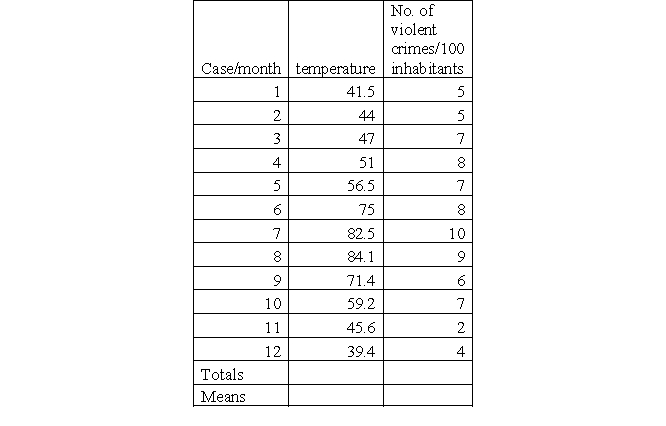
Academic literature found evidence that there is a relationship between temperature and the frequency of the occurrence of violent crimes. Utilizing data derived from the local police department (number of violent crimes/month/100 inhabitants) and meteorological data (average temperature/month), you want to determine the relationship between temperature (IV) and the frequency of violent crime (DV). Find the distribution of both variables in the table below.
a. Use a spreadsheet program to create a scatterplot or draw it by hand. Describe what you see.
b. Compute beta (b) and interpret your result.
c. Compute the constant (a) and interpret your result.
d. Assume you want to predict the frequency of violent crimes in a month with an average temperature of 90.5 degrees Fahrenheit. Compute y.
To predict a certain outcome having detailed knowledge about the independent variable, which is impacting the dependent variable, the most appropriate statistical test to run is
It is debated whether IQ scores influence criminal behavior (either directly or indirectly). It is argued that the majority of criminals have an IQ that lies 8 points below (92) the average IQ (100). You draw a random sample of 15 individuals of age 18+, assess the IQ of participants, and ask them about their criminal history (number of offenses committed, not including minor traffic violations). You select an alpha of 0.05. The results of your assessment are to be found in the table presented below.
a. State your null and alternative hypotheses.
b. State your decision rule to determine statistical significance.
c. Utilizing the data from the table presented below:
i. Compute beta (b).
ii. Compute the constant (a).
iii. Determine the strength and direction of the relationship by computing Pearson's r.
iv. Compute r2.
v. Compute the prediction error you could possibly have if you know nothing about the distribution of the independent variable (IQ score).
vi. Compute the unexplained variance.
vii. Compute the explained variance.
d. Make a decision.
e. Compute the standard error of estimate.
f. INTERPRET ALL YOUR RESULTS.
Case IQ (x) No. of offenses (y) 1 90 4 2 110 1 3 89 4 4 95 3 5 92 5 6 91 4 7 102 0 8 99 2 9 76 3 10 99 1 11 92 6 12 98 1 13 111 1 14 100 2 15 93 6
Using the example from problem 2:
a. State your null and your alternative hypotheses.
b. Determine the strength and direction of the relationship by computing Pearson's r. Interpret your results.
c. Compute r2 and interpret your result.
To warm up, let us start with a problem that has a "perfect" regression line. Assume that the state prison wants to encourage prisoners to get involved in education. Thus, the prison administration offers that for every hour spent on education, inmates receive 5 additional minutes in the prison yard.
a. Compute beta and interpret your finding.
b. Compute the constant (y intercept or a) and interpret your finding.
y 0 0 1 5 2 10 3 15 4 20 5 25 6 30 7 35 8 40 9 45 10 50 Totals Means
c. Assume that John (inmate) has studied 17 hours in the previous week; how many minutes of additional yard time did he earn? Use the classic algebraic equation (y = a + bx) to calculate the amount of minutes earned and interpret your result.
d. Next, you want to predict the total time an inmate is allowed to spend in the yard (weekly allowance + additional time earned). The weekly allowance regarding yard time is (without additional time earned) 630 minutes (10.5 hours).
x y 0 630 1 635 2 640 3 645 4 650 5 655 6 660 7 665 8 670 9 675 10 680 Totals Means
i. Compute beta.
ii. Compute the constant (a or y-intercept).
iii. How many minutes (total) is John allowed to spend in the prison yard if he has studied for 21 hours? Use the classic algebraic equation (y = a + bx).
Many formulas utilized in statistics are complex. However, one basic formula used in regression is a classic algebraic equation: y = a + bx. Explain the variables within this formula.
Filters
- Essay(0)
- Multiple Choice(0)
- Short Answer(0)
- True False(0)
- Matching(0)