Exam 8: Basic Macroeconomic Relationships
Exam 1: Limits, Alternatives, and Choices261 Questions
Exam 2: The Market System and the Circular Flow112 Questions
Exam 4: Introduction to Macroeconomics58 Questions
Exam 5: Measuring the Economys Output183 Questions
Exam 6: Economic Growth113 Questions
Exam 7: Business Cycles, Unemployment, and Inflation184 Questions
Exam 8: Basic Macroeconomic Relationships188 Questions
Exam 9: The Aggregate Expenditures Model235 Questions
Exam 10: Aggregate Demand and Aggregate Supply195 Questions
Exam 11: Fiscal Policy, Deficits, Surpluses, and Debt223 Questions
Exam 12: Money, Banking, and Money Creation286 Questions
Exam 13: Interest Rates and Monetary Policy376 Questions
Exam 14: Financial Economics51 Questions
Exam 15: Long-Run Macroeconomic Adjustments122 Questions
Exam 16: International Trade181 Questions
Exam 17: Exchange Rates and the Balance of Payments127 Questions
Select questions type
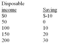
Given the consumption schedule, it is possible to graph the relevant saving schedule by:
(Multiple Choice)
4.9/5  (37)
(37)
 -Refer to the above data. The marginal propensity to consume is:
(Multiple Choice)
4.7/5 (38)
If business taxes are reduced and the real interest rate increases:
(Multiple Choice)
4.9/5 (35)
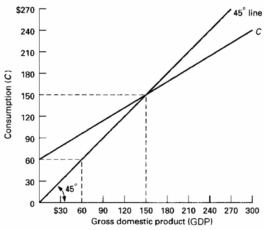
At the point where the consumption schedule intersects the 45-degree line:
(Multiple Choice)
4.8/5 (38)
Suppose the consumption schedule is: C = 20 + .9Y, where C is consumption and Y is disposable income.
-Refer to the above data. The MPC is:
(Multiple Choice)
4.9/5 (41)
Following is consumption schedules for three private closed economies. DI signifies disposable income and C represents consumption expenditures. All figures are in billions of dollars. Refer to the data below. Suppose the consumption is increased by $2 billion in each of the three economies. This change could have been caused by: 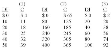
(Multiple Choice)
5.0/5 (39)
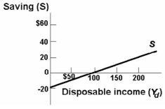
 -Refer to the above diagram. The equation for the saving schedule is:
(Multiple Choice)
4.8/5 (30)
-Refer to the above data. At the $100 level of income, the average propensity to save is:
(Multiple Choice)
4.8/5 (33)
The ________ of the late 1990s was an example of the wealth effect, while _______ of 2008 was an example of the reverse wealth effect.
(Multiple Choice)
4.9/5 (42)
Other things equal, the real interest rate and the level of investment are:
(Multiple Choice)
4.9/5 (35)
 -Refer to the above diagram. The break-even level of disposable income:
(Multiple Choice)
4.8/5 (43)
Holly's break-even level of income is $10,000 and her MPC is 0.75. If her actual disposable income is $16,000, her level of:
(Multiple Choice)
4.8/5 (38)
The initial costs of capital goods, and the estimated costs of operating and maintaining those goods, affect the expected rate of return on investment.
(True/False)
5.0/5 (41)
If the MPC is .70 and gross investment increases by $3 billion, the equilibrium GDP will:
(Multiple Choice)
4.8/5 (38)
Following is consumption schedules for three private closed economies. DI signifies disposable income and C represents consumption expenditures. All figures are in billions of dollars.
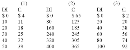 -Refer to the above data. The marginal propensity to consume:
(Multiple Choice)
4.9/5 (36)
Filters
- Essay(0)
- Multiple Choice(0)
- Short Answer(0)
- True False(0)
- Matching(0)