Exam 11: Regression Analysis: Statistical Inference
(A)Estimate a simple linear regression model using the sample data.How well does the estimated model fit the sample data?
(B)Perform an F-test for the existence of a linear relationship between Y and X.Use a 5% level of significance.
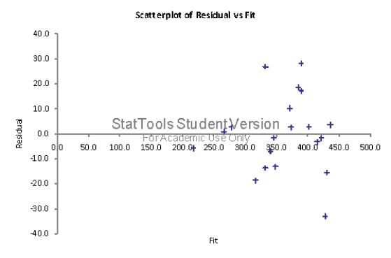
(C)Plot the fitted values versus residuals associated with the model in Question 119.What does the plot indicate?
(D)How do you explain the results you have found in (A)through (C)?
(E)Suppose you learn that the 10th employee in the sample has been fired for missing an excessive number of work-hours during the past year.In light of this information,how would you proceed to estimate the relationship between the number of work-hours an employee misses per year and the employee's annual wages,using the available information? If you decide to revise your estimate of this regression equation,repeat (A)and (B)
(A) 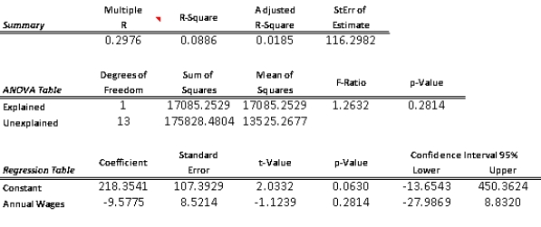 The simple linear regression model is
  =218.35 - 9.5775 (Annual Wages).The fit of this estimated model is pretty poor; the percent variation explained is only 0.0886.(B)Since the p-value = 0.2814 is well above 0.05,this indicates that there is no linear relationship between Y (work hours missed)and X (employee's annual wages).(C)
 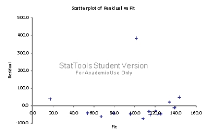 The chart of residuals versus fitted values points to an obvious outlier associated with the 10th employee in the sample who has missed 485 hours of work (for this employee,fitted value = 101.5 and residual = 383.5).(D)Since there is no evidence of a linear relationship between X and Y,and the existence of an obvious outlier,the estimated linear regression model in (A)provides a very poor fit to the data.(E)We should eliminate the data point associated with this employee and rerun the regression in (A)and (B).We expect to obtain much better results.
 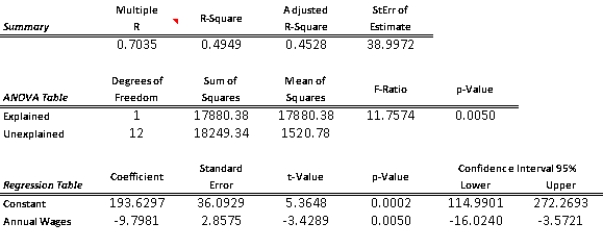 The simple linear regression model is
  =193.6 - 9.79 (Annual Wages).The fit of this estimated model is much better than the one obtained in (A).The percentage of variation explained has improved from only 0.0886 to 0.4949.In addition,with the revised model,the p-value = 0.005 is well below 0.05,which indicates that there is a linear relationship between Y (work hours missed)and X (employee's annual wages).This also confirms what we expect to see,intuitively; as wages increase,worker hours missed decreases (i.e.,slope is negative).
In order to estimate with 90% confidence a particular value of Y for a given value of X in a simple linear regression problem,a random sample of 20 observations is taken.The appropriate t-value that would be used is 1.734.
True
Suggest an alternative model to address the issues identified in Question 131.Are you able to obtain an improved fit to the data? Explain your answer.
Since a logarithmic transformation can often address both slight non-linearity and heteroskedasticity,we might first try transforming the X variable,Ad Data.Following are the regression results in that case: 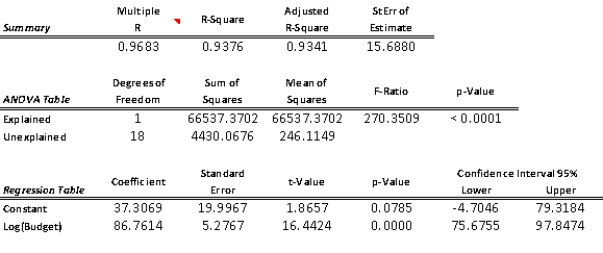
 The fit of this model on the log-transformed data is much better than the one obtained in Question 128.The percentage of variation explained has improved to almost 94% and we have a much better looking residuals plot as well,with no apparent pattern.
One method of dealing with heteroscedasticity is to try a logarithmic transformation of the data.
In regression analysis,the unexplained part of the total variation in the response variable Y is referred to as sum of squares due to regression,SSR.
One of the potential characteristics of an outlier is that the value of the dependent variable is much larger or smaller than predicted by the regression line.
Determining which variables to include in regression analysis by estimating a series of regression equations by successively adding or deleting variables according to prescribed rules is referred to as:
The Durbin-Watson statistic can be used to measure of autocorrelation.
(A)Estimate the regression model.How well does this model fit the given data?
(B)Is there a linear relationship between X and Y at the 5% significance level? Explain how you arrived at your answer.
(C)Use the estimated regression model to predict the number of caps that will be sold during the next month if the average selling price is $10.
(D)Find a 95% prediction interval for the number of caps determined in Question 90.Use t- multiple = 2.
(E)Find a 95% confidence interval for the average number of caps sold given an average selling price of $10.Use a t-multiple = 2.
(F)How do you explain the differences between the widths of the intervals in (D)and (E)?
(A)Estimate a multiple regression model that includes the two given explanatory variables.Assess this set of explanatory variables with an F-test,and report a p-value.
(B)Conduct a partial F-test to decide whether it is worthwhile to add second-order terms (i.e.,  )to the multiple regression equation estimated in Question 114.Employ a 5% significance level in conducting this hypothesis test.
(C)Identify and interpret the percentage of variance explained for the model in (A).
(D)Identify and interpret the percentage of variance explained for the model in (B).
(E)Which regression equation is the most appropriate one for modeling the quality of the given product? Bear in mind that a good statistical model is usually parsimonious.
)to the multiple regression equation estimated in Question 114.Employ a 5% significance level in conducting this hypothesis test.
(C)Identify and interpret the percentage of variance explained for the model in (A).
(D)Identify and interpret the percentage of variance explained for the model in (B).
(E)Which regression equation is the most appropriate one for modeling the quality of the given product? Bear in mind that a good statistical model is usually parsimonious.
Diagnose what may be causing the problem seen in the residuals plot in Question 130.What issue(s)do you identify?
The error term represents the vertical distance from any point to the
In multiple regressions,a large value of the test statistic F indicates that most of the variation in Y is unexplained by the regression equation and that the model is useless.A small value of F indicates that most of the variation in Y is explained by the regression equation and that the model is useful.
Which of the following is not one of the guidelines for including/excluding variables in a regression equation?
The value of the sum of squares due to regression,SSR,can never be larger than the value of the sum of squares total,SST.
In regression analysis,homoscedasticity refers to constant error variance.
Filters
- Essay(0)
- Multiple Choice(0)
- Short Answer(0)
- True False(0)
- Matching(0)