Short Answer
TABLE 15-9
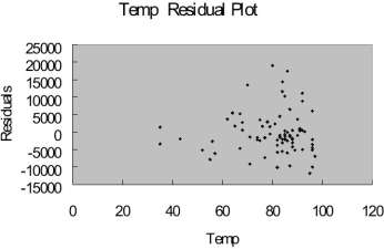
Many factors determine the attendance at Major League Baseball games. These factors can include when the game is played, the weather, the opponent, whether or not the team is having a good season, and whether or not a marketing promotion is held. Data from 80 games of the Kansas City Royals for the following variables are collected.
ATTENDANCE = Paid attendance for the game
TEMP = High temperature for the day
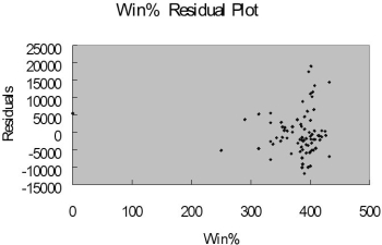
WIN% = Team's winning percentage at the time of the game
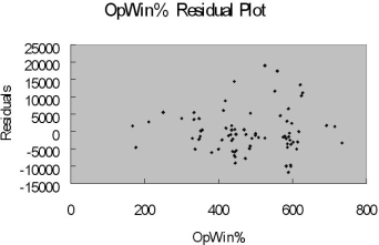
OPWIN% = Opponent team's winning percentage at the time of the game WEEKEND - 1 if game played on Friday, Saturday or Sunday; 0 otherwise PROMOTION - 1 = if a promotion was held; 0 = if no promotion was held
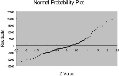
The regression results using attendance as the dependent variable and the remaining five variables as the independent variables are presented below.
The coefficient of multiple determination ( R 2 j ) of each of the 5 predictors with all the other remaining predictors are,
respectively, 0.2675, 0.3101, 0.1038, 0.7325, and 0.7308.
-Referring to Table 15-9,_____ of the variation in ATTENDANCE can be explained by the five independent variables after taking into consideration the number of independent variables and the number of observations.
Correct Answer:

Verified
Correct Answer:
Verified
Q2: TABLE 15- 8<br>The superintendent of a
Q3: TABLE 15-7<br>A chemist employed by a
Q4: TABLE 15-3<br>A certain type of rare
Q7: TABLE 15-7<br>A chemist employed by a
Q8: TABLE 15-9<br>Many factors determine the attendance
Q11: TABLE 15-4<br>In Hawaii, condemnation proceedings are
Q13: A regression diagnostic tool used to study
Q33: TABLE 15-9<br>Many factors determine the attendance
Q52: Collinearity is present when there is a
Q63: Collinearity will result in excessively low standard