Exam 17: Getting Ready to Analyze Data

SCENARIO 17-1 A real estate builder wishes to determine how house size (House) is influenced by family income (Income), family size (Size), and education of the head of household (School). House size is measured in hundreds of square feet, income is measured in thousands of dollars, and education is in years. The builder randomly selected 50 families and ran the multiple regression. Microsoft Excel output is provided below: SUMMARY OUTPUT Regression Statistics Multiple R 0.865 R Square 0.748 Adjusted R Square 0.726 Standard Error 5.195 Observations 50 ANOVA df SS MS F Signif F Regression 3605.7736 1201.9245 0.0000 Residual 1214.2264 26.3962 Total 49 4820.0000 Coeff StdError t Stat P -value Intercept -1.6335 5.8078 -0.281 0.7798 Income 0.4485 0.1137 3.9545 0.0003 Size 4.2615 0.8062 5.286 0.0001 School -0.6517 0.4319 -1.509 0.1383 -Referring to Scenario 17-1, which of the following values for the level of significance is the smallest for which the regression model as a whole is significant?

Double-clicking a cell in a PivotTable causes Excel to drill down and display the underlying data in a new worksheet.

SCENARIO 17-8 The superintendent of a school district wanted to predict the percentage of students passing a sixth- grade proficiency test. She obtained the data on percentage of students passing the proficiency test (% Passing), daily mean of the percentage of students attending class (% Attendance), mean teacher salary in dollars (Salaries), and instructional spending per pupil in dollars (Spending) of 47 schools in the state. Following is the multiple regression output with $Y = \%$ Passing as the dependent variable, $X _ { 1 } = \%$ Attendance, $X _ { 2 } =$ Salaries and $X _ { 3 } =$ Spending: Regression Statistics Multiple R 0.7930 R Square 0.6288 Adjusted R 0.6029 Square Standard 10.4570 Error Observations 47 ANOVA Coefficients Standard Error t Stat P-value Lower 95\% Upper 95\% Intercept -753.4225 101.1149 -7.4511 0.0000 -957.3401 -549.5050 \% Attendance 8.5014 1.0771 7.8929 0.0000 6.3292 10.6735 Salary 0.000000685 0.0006 0.0011 0.9991 -0.0013 0.0013 Spending 0.0060 0.0046 1.2879 0.2047 -0.0034 0.0153 -Referring to Scenario 17-8, what is the value of the test statistic when testing whether instructional spending per pupil has any effect on percentage of students passing the proficiency test, taking into account the effect of all the other independent variables?

SCENARIO 17-8 The superintendent of a school district wanted to predict the percentage of students passing a sixth- grade proficiency test. She obtained the data on percentage of students passing the proficiency test (% Passing), daily mean of the percentage of students attending class (% Attendance), mean teacher salary in dollars (Salaries), and instructional spending per pupil in dollars (Spending) of 47 schools in the state. Following is the multiple regression output with $Y = \%$ Passing as the dependent variable, $X _ { 1 } = \%$ Attendance, $X _ { 2 } =$ Salaries and $X _ { 3 } =$ Spending: Regression Statistics Multiple R 0.7930 R Square 0.6288 Adjusted R 0.6029 Square Standard 10.4570 Error Observations 47 ANOVA Coefficients Standard Error t Stat P-value Lower 95\% Upper 95\% Intercept -753.4225 101.1149 -7.4511 0.0000 -957.3401 -549.5050 \% Attendance 8.5014 1.0771 7.8929 0.0000 6.3292 10.6735 Salary 0.000000685 0.0006 0.0011 0.9991 -0.0013 0.0013 Spending 0.0060 0.0046 1.2879 0.2047 -0.0034 0.0153 -Referring to Scenario 17-8, the null hypothesis $H _ { 0 } : \beta _ { 1 } = \beta _ { 2 } = \beta _ { 3 } = 0$ implies that percentage of students passing the proficiency test is not affected by any of the explanatory variables.

SCENARIO 17-1 A real estate builder wishes to determine how house size (House) is influenced by family income (Income), family size (Size), and education of the head of household (School). House size is measured in hundreds of square feet, income is measured in thousands of dollars, and education is in years. The builder randomly selected 50 families and ran the multiple regression. Microsoft Excel output is provided below: SUMMARY OUTPUT Regression Statistics Multiple R 0.865 R Square 0.748 Adjusted R Square 0.726 Standard Error 5.195 Observations 50 ANOVA df SS MS F Signif F Regression 3605.7736 1201.9245 0.0000 Residual 1214.2264 26.3962 Total 49 4820.0000 Coeff StdError t Stat P -value Intercept -1.6335 5.8078 -0.281 0.7798 Income 0.4485 0.1137 3.9545 0.0003 Size 4.2615 0.8062 5.286 0.0001 School -0.6517 0.4319 -1.509 0.1383 -Referring to Scenario 17-1, which of the following values for the level of significance is the smallest for which at least two explanatory variables are significant individually?

SCENARIO 17-12 The marketing manager for a nationally franchised lawn service company would like to study the characteristics that differentiate home owners who do and do not have a lawn service. A random sample of 30 home owners located in a suburban area near a large city was selected; 15 did not have a lawn service (code 0) and 15 had a lawn service (code 1). Additional information available concerning these 30 home owners includes family income (Income, in thousands of dollars), lawn size (Lawn Size, in thousands of square feet), attitude toward outdoor recreational activities (Atitude 0 = unfavorable, 1 = favorable), number of teenagers in the household (Teenager), and age of the head of the household (Age). The Minitab output is given below: 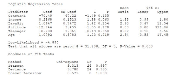-Referring to Scenario 17-12, what should be the decision ('reject' or 'do not reject') on the null hypothesis when testing whether LawnSize makes a significant contribution to the model in the presence of the other independent variables at a 0.05 level of significance?

SCENARIO 17-1 A real estate builder wishes to determine how house size (House) is influenced by family income (Income), family size (Size), and education of the head of household (School). House size is measured in hundreds of square feet, income is measured in thousands of dollars, and education is in years. The builder randomly selected 50 families and ran the multiple regression. Microsoft Excel output is provided below: SUMMARY OUTPUT Regression Statistics Multiple R 0.865 R Square 0.748 Adjusted R Square 0.726 Standard Error 5.195 Observations 50 ANOVA df SS MS F Signif F Regression 3605.7736 1201.9245 0.0000 Residual 1214.2264 26.3962 Total 49 4820.0000 Coeff StdError t Stat P -value Intercept -1.6335 5.8078 -0.281 0.7798 Income 0.4485 0.1137 3.9545 0.0003 Size 4.2615 0.8062 5.286 0.0001 School -0.6517 0.4319 -1.509 0.1383 -Referring to Scenario 17-1, what minimum annual income would an individual with a family size of 9 and 10 years of education need to attain a predicted 5,000 square foot home (House = 50)?

The director of admissions at a state college is interested in seeing if admissions status (admitted, waiting list, denied admission) at his college is related to the type of community (urban, rural, Suburban) in which an applicant resides. Which of the following tests will be the most Appropriate?

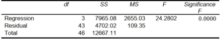
SCENARIO 17-5 You worked as an intern at We Always Win Car Insurance Company last summer. You notice that individual car insurance premiums depend very much on the age of the individual, the number of traffic tickets received by the individual, and the population density of the city in which the individual lives. You performed a regression analysis in EXCEL and obtained the following information: Regression Statistics Multiple R 0.63 R Square 0.40 Adjusted R Square 0.23 Standard Error 50.00 Observations 15.00 ANOVA df SS MS F Significance F Regression 3 5994.24 2.40 0.12 Residual 11 27496.82 Total 45479.54 Coefficients Standard Error t Stat P-value Lower 99.0\% Upper 99.0\% Intercept 123.80 48.71 2.54 0.03 -27.47 275.07 AGE -0.82 0.87 -0.95 0.36 -3.51 1.87 TICKETS 21.25 10.66 1.99 0.07 -11.86 54.37 DENSITY -3.14 6.46 -0.49 0.64 -23.19 16.91 AGE -0.82 0.87 -0.95 0.36 -3.51 1.87 TICKETS 21.25 10.66 1.99 0.07 -11.86 54.37 DENSITY -3.14 6.46 -0.49 0.64 -23.19 16.91 -Referring to Scenario 17-5, the total degrees of freedom that are missing in the ANOVA table should be ______.

SCENARIO 17-8 The superintendent of a school district wanted to predict the percentage of students passing a sixth- grade proficiency test. She obtained the data on percentage of students passing the proficiency test (% Passing), daily mean of the percentage of students attending class (% Attendance), mean teacher salary in dollars (Salaries), and instructional spending per pupil in dollars (Spending) of 47 schools in the state. Following is the multiple regression output with $Y = \%$ Passing as the dependent variable, $X _ { 1 } = \%$ Attendance, $X _ { 2 } =$ Salaries and $X _ { 3 } =$ Spending: Regression Statistics Multiple R 0.7930 R Square 0.6288 Adjusted R 0.6029 Square Standard 10.4570 Error Observations 47 ANOVA Coefficients Standard Error t Stat P-value Lower 95\% Upper 95\% Intercept -753.4225 101.1149 -7.4511 0.0000 -957.3401 -549.5050 \% Attendance 8.5014 1.0771 7.8929 0.0000 6.3292 10.6735 Salary 0.000000685 0.0006 0.0011 0.9991 -0.0013 0.0013 Spending 0.0060 0.0046 1.2879 0.2047 -0.0034 0.0153 -Referring to Scenario 17-8, you can conclude that mean teacher salary individually has no impact on the mean percentage of students passing the proficiency test, taking into account the effect of all the other independent variables, at a 1% level of significance based solely on the 95% confidence interval estimate for $\beta _ { 2 }$ .

SCENARIO 17-10 Given below are results from the regression analysis where the dependent variable is the number of weeks a worker is unemployed due to a layoff (Unemploy) and the independent variables are the age of the worker (Age), the number of years of education received (Edu), the number of years at the previous job (Job Yr), a dummy variable for marital status (Married: $1 =$ married, $0 =$ otherwise), a dummy variable for head of household (Head: $1 =$ yes, $0 =$ no) and a dummy variable for management position (Manager: $1 =$ yes, $0 =$ no). We shall call this Model 1. The coefficient of partial determination ( $R _ { \mathrm { y } } ^ { 2 }$ (All raiables excopt $j$ ) ) of each of the 6 predictors are, respectively, $0.2807$ , $0.0386,0.0317,0.0141,0.0958$ , and $0.1201$ . Regression Statistics Multiple R 0.7035 R Square 0.4949 Adjusted R 0.4030 Square Standard 18.4861 Error Observations 40 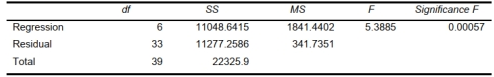$\text { ANOVA }$ Coefficients Standard Error t Stat P-value Lower 95\% Upper 95\% Intercept 32.6595 23.18302 1.4088 0.1683 -14.5067 79.8257 Age 1.2915 0.3599 3.5883 0.0011 0.5592 2.0238 Edu -1.3537 1.1766 -1.1504 0.2582 -3.7476 1.0402 Job Yr 0.6171 0.5940 1.0389 0.3064 -0.5914 1.8257 Married -5.2189 7.6068 -0.6861 0.4974 -20.6950 10.2571 Head -14.2978 7.6479 -1.8695 0.0704 -29.8575 1.2618 Manager -24.8203 11.6932 -2.1226 0.0414 -48.6102 -1.0303 -Referring to Scenario 17-10 Model 1, the null hypothesis should be rejected at a 10% level of significance when testing whether age has any effect on the number of weeks a worker is unemployed due to a layoff.

The superintendent of a school district wanted to predict the percentage of students passing a sixth-grade proficiency test. She obtained the data on percentage of students passing the Proficiency test (% Passing), daily mean of the percentage of students attending class (% Attendance), mean teacher salary in dollars (Salaries), and instructional spending per pupil in Dollars (Spending) of 47 schools in the state. She believed that holding everything else constant, Instructional spending per pupil had a positive but decreasing impact on percentage. Which of The following would be the most appropriate analysis to perform?

SCENARIO 17-10 Given below are results from the regression analysis where the dependent variable is the number of weeks a worker is unemployed due to a layoff (Unemploy) and the independent variables are the age of the worker (Age), the number of years of education received (Edu), the number of years at the previous job (Job Yr), a dummy variable for marital status (Married: $1 =$ married, $0 =$ otherwise), a dummy variable for head of household (Head: $1 =$ yes, $0 =$ no) and a dummy variable for management position (Manager: $1 =$ yes, $0 =$ no). We shall call this Model 1. The coefficient of partial determination ( $R _ { \mathrm { y } } ^ { 2 }$ (All raiables excopt $j$ ) ) of each of the 6 predictors are, respectively, $0.2807$ , $0.0386,0.0317,0.0141,0.0958$ , and $0.1201$ . Regression Statistics Multiple R 0.7035 R Square 0.4949 Adjusted R 0.4030 Square Standard 18.4861 Error Observations 40 $\text { ANOVA }$ Coefficients Standard Error t Stat P-value Lower 95\% Upper 95\% Intercept 32.6595 23.18302 1.4088 0.1683 -14.5067 79.8257 Age 1.2915 0.3599 3.5883 0.0011 0.5592 2.0238 Edu -1.3537 1.1766 -1.1504 0.2582 -3.7476 1.0402 Job Yr 0.6171 0.5940 1.0389 0.3064 -0.5914 1.8257 Married -5.2189 7.6068 -0.6861 0.4974 -20.6950 10.2571 Head -14.2978 7.6479 -1.8695 0.0704 -29.8575 1.2618 Manager -24.8203 11.6932 -2.1226 0.0414 -48.6102 -1.0303 -Referring to Scenario 17-10 Model 1, which of the following is the correct alternative hypothesis to test whether age has any effect on the number of weeks a worker is unemployed Due to a layoff while holding constant the effect of all the other independent variables? a) $H _ { 1 } : \beta _ { 0 } \neq 0$ b) $H _ { 1 } : \beta _ { 1 } \neq 0$ c) $H _ { 1 } : \beta _ { 2 } \neq 0$ d) $H _ { 1 } : \beta _ { 3 } \neq 0$

An entrepreneur is considering the purchase of a coin-operated laundry. The current owner claims that over the past 5 years, the mean daily revenue was $675 with a standard deviation of $75. A Sample of 30 days reveals a daily mean revenue of $625 and a standard deviation of $70. Which Of the following tests will be the most appropriate?

Which of the following is NOT one of the categories of predictive analytics methods?

SCENARIO 17-12 The marketing manager for a nationally franchised lawn service company would like to study the characteristics that differentiate home owners who do and do not have a lawn service. A random sample of 30 home owners located in a suburban area near a large city was selected; 15 did not have a lawn service (code 0) and 15 had a lawn service (code 1). Additional information available concerning these 30 home owners includes family income (Income, in thousands of dollars), lawn size (Lawn Size, in thousands of square feet), attitude toward outdoor recreational activities (Atitude 0 = unfavorable, 1 = favorable), number of teenagers in the household (Teenager), and age of the head of the household (Age). The Minitab output is given below: -Referring to Scenario 17-12, there is not enough evidence to conclude that Teenager makes a significant contribution to the model in the presence of the other independent variables at a 0.05 level of significance.

SCENARIO 17-10 Given below are results from the regression analysis where the dependent variable is the number of weeks a worker is unemployed due to a layoff (Unemploy) and the independent variables are the age of the worker (Age), the number of years of education received (Edu), the number of years at the previous job (Job Yr), a dummy variable for marital status (Married: $1 =$ married, $0 =$ otherwise), a dummy variable for head of household (Head: $1 =$ yes, $0 =$ no) and a dummy variable for management position (Manager: $1 =$ yes, $0 =$ no). We shall call this Model 1. The coefficient of partial determination ( $R _ { \mathrm { y } } ^ { 2 }$ (All raiables excopt $j$ ) ) of each of the 6 predictors are, respectively, $0.2807$ , $0.0386,0.0317,0.0141,0.0958$ , and $0.1201$ . Regression Statistics Multiple R 0.7035 R Square 0.4949 Adjusted R 0.4030 Square Standard 18.4861 Error Observations 40 $\text { ANOVA }$ Coefficients Standard Error t Stat P-value Lower 95\% Upper 95\% Intercept 32.6595 23.18302 1.4088 0.1683 -14.5067 79.8257 Age 1.2915 0.3599 3.5883 0.0011 0.5592 2.0238 Edu -1.3537 1.1766 -1.1504 0.2582 -3.7476 1.0402 Job Yr 0.6171 0.5940 1.0389 0.3064 -0.5914 1.8257 Married -5.2189 7.6068 -0.6861 0.4974 -20.6950 10.2571 Head -14.2978 7.6479 -1.8695 0.0704 -29.8575 1.2618 Manager -24.8203 11.6932 -2.1226 0.0414 -48.6102 -1.0303 -Referring to Scenario 17-10 Model 1, the alternative hypothesis H1 : At least one of ?j ? 0 for j = 1, 2, 3, 4, 5, 6 implies that the number of weeks a worker is unemployed due to a layoff is affected by at least one of the explanatory variables.

SCENARIO 17-1 A real estate builder wishes to determine how house size (House) is influenced by family income (Income), family size (Size), and education of the head of household (School). House size is measured in hundreds of square feet, income is measured in thousands of dollars, and education is in years. The builder randomly selected 50 families and ran the multiple regression. Microsoft Excel output is provided below: SUMMARY OUTPUT Regression Statistics Multiple R 0.865 R Square 0.748 Adjusted R Square 0.726 Standard Error 5.195 Observations 50 ANOVA df SS MS F Signif F Regression 3605.7736 1201.9245 0.0000 Residual 1214.2264 26.3962 Total 49 4820.0000 Coeff StdError t Stat P -value Intercept -1.6335 5.8078 -0.281 0.7798 Income 0.4485 0.1137 3.9545 0.0003 Size 4.2615 0.8062 5.286 0.0001 School -0.6517 0.4319 -1.509 0.1383 -Referring to Scenario 17-1, what is the predicted house size (in hundreds of square feet) for an individual earning an annual income of $40,000, having a family size of 4, and going to school a Total of 13 years?

Some business analytics involve starting with many variables, followed by filtering the data by exploring specific combinations of categorical values or numerical range. In Excel, this approach is mimicked by using a slicer.

Suppose that past history shows that 6% of college students prefer Brand A Cola. A sample of 10,000 students is to be selected. Which of the following distributions would you use to compute The probability that at least half of them will prefer Brand A cola?