Exam 14: Inference for Regression
Exam 1: Data and Decisions41 Questions
Exam 2: Displaying and Describing Categorical Data45 Questions
Exam 3: Displaying and Describing Quantitative Data32 Questions
Exam 4: Correlation and Linear Regression84 Questions
Exam 5: Randomness and Probability34 Questions
Exam 6: Random Variables and Probability Models28 Questions
Exam 7: The Normal and Other Continuous Distributions31 Questions
Exam 8: Surveys and Sampling30 Questions
Exam 9: Sampling Distributions and Confidence Intervals for Proportions66 Questions
Exam 10: Testing Hypotheses About Proportions27 Questions
Exam 11: Confidence Intervals and Hypothesis Tests for Means28 Questions
Exam 12: Comparing Two Means35 Questions
Exam 13: Inference for Counts: Chi-Square Tests68 Questions
Exam 14: Inference for Regression38 Questions
Exam 15: Multiple Regression36 Questions
Exam 16: Introduction to Data Mining68 Questions
Select questions type
Consider Scatterplots 1 and 2 with fitted regression lines shown below. Which of the following statements is true? 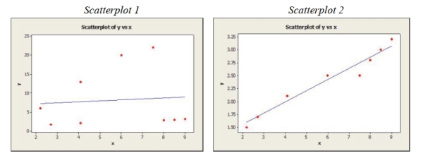
(Multiple Choice)
4.8/5  (24)
(24)
When using a plot of residuals (y-axis) vs. fitted value of the dependent variable, a plot with no pattern indicates that the:
(Multiple Choice)
4.8/5 (32)
Use the following for questions
A sales manager was interested in determining if there is a relationship between college GPA and sales performance among salespeople hired within the last year. A sample of recently hired salespeople was selected and college GPA and the number of units sold last month recorded. Below are the scatterplot, regression results, and residual plots for these data. The regression equation is
Units Sold GPA
Predictor Coef SE Coef T P Constant -0.484 3.256 -0.15 0.884 GPA 7.423 1.044 7.11 0.000
Analysis of Variance
Source DF SS MS F P Regression 1 125.30 125.30 50.56 0.000 Residual Error 14 34.70 2.48 Total 15 160.00 Answer: 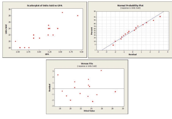 -Test the hypotheses about the slope of the regression line. Give the appropriate test
statistic, associated P-value, and conclusion in terms of the problem.
-Test the hypotheses about the slope of the regression line. Give the appropriate test
statistic, associated P-value, and conclusion in terms of the problem.
(Essay)
4.7/5 (38)
A sample of recently trained line workers was selected to determine if there is a relationship between the number of hours of training time received by production line Workers and the time it took (in minutes) for them to trouble shoot their last process Problem were captured. Using the regression output is shown below, what conclusion Should be made at α = .05? The regression equation is Trouble Shooting Training
Predictor Coef SE Coef T Constant 30.729 1.023 30.03 0.000 Training -1.8360 0.1376 -13.35 0.000
(Multiple Choice)
4.8/5 (33)
The following plots show (1) world population (millions) plotted against 5-year intervals from 1950 through 2000 and (2) residual vs. fitted value for a linear regression model estimated to describe the trend in world population over time. Based on these plots, would you consider this model appropriate? Explain.
(Essay)
4.8/5 (32)
Use the following for questions
A sales manager was interested in determining if there is a relationship between college GPA and sales performance among salespeople hired within the last year. A sample of recently hired salespeople was selected and college GPA and the number of units sold last month recorded. Below are the scatterplot, regression results, and residual plots for these data. The regression equation is
Units Sold GPA
Predictor Coef SE Coef T P Constant -0.484 3.256 -0.15 0.884 GPA 7.423 1.044 7.11 0.000
Analysis of Variance
Source DF SS MS F P Regression 1 125.30 125.30 50.56 0.000 Residual Error 14 34.70 2.48 Total 15 160.00 Answer:
-What percentage of the variability in sales performance (units sold per month) can be
accounted for by college GPA?
(Essay)
4.7/5 (33)
Use the following for questions
A sales manager was interested in determining if there is a relationship between college GPA and sales performance among salespeople hired within the last year. A sample of recently hired salespeople was selected and college GPA and the number of units sold last month recorded. Below are the scatterplot, regression results, and residual plots for these data. The regression equation is
Units Sold GPA
Predictor Coef SE Coef T P Constant -0.484 3.256 -0.15 0.884 GPA 7.423 1.044 7.11 0.000
Analysis of Variance
Source DF SS MS F P Regression 1 125.30 125.30 50.56 0.000 Residual Error 14 34.70 2.48 Total 15 160.00 Answer:
-Predict the units sold per month for a new hire whose college GPA is 3.00.
(Essay)
4.9/5 (35)
The number of hours of training time received by employees and the time it took (in minutes) for them to trouble shoot their last process problem was estimated using a
Regression equation. The 95% prediction interval for trouble shooting time with 8
Hours of training was determined to be 12.822 to 19.261. The correct interpretation is
(Multiple Choice)
4.8/5 (38)
As the carbon content in steel increases, its ductility tends to decrease. A researcher at a steel company measures carbon content and ductility for a sample of 15 types of
Steel. According to the output provided below, the standard error of the regression
Slope is The regression equation is
Ductility Carbon Content
Predictor Coef SE Coef T P Constant 7.671 1.507 5.09 0.000 Carbon Content -3.296 1.097 -3.01 0.010
(Multiple Choice)
4.8/5 (38)
Data on labor productivity and unit labor costs were obtained for the retail industry from 1987 through 2006 (Bureau of Labor Statistics). A regression was estimated to describe the linear relationship between the two variables. Based on the plot of residuals versus predicted values, is the linear model appropriate? Explain.
(Essay)
4.9/5 (37)
Use the following for questions
An operations manager was interested in determining if there is a relationship between the amount of training received by production line workers and the time it takes for them to troubleshoot a process problem. A sample of recently trained line workers was selected. The number of hours of training time received and the time it took (in minutes) for them to troubleshoot their last process problem were captured. Below are the scatterplot, regression results, and residual plots for these data. The regression equation is
Trouble Shooting Training
Predictor Coef SE Coef T P Constant 30.729 1.023 30.03 0.000 Training -1.8360 0.1376 -13.35 0.000
Analysis of Variance
Source DF SS MS F P Regression 1 367.20 367.20 178.10 0.000 Residual Error 13 26.80 2.06 Total 14 394.00
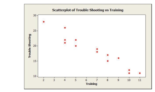 -According to the data, a worker who received 8 hours of training had a
troubleshooting time of 15 minutes. What is the value of the residual for this worker?
Explain what the residual means.
-According to the data, a worker who received 8 hours of training had a
troubleshooting time of 15 minutes. What is the value of the residual for this worker?
Explain what the residual means.
(Essay)
4.7/5 (29)
A sales manager claims that there is a relationship between college GPA and sales performance (number of units sold) among salespeople hired within the last year.
Use the regression results are shown below and set α = .05 to test his claim. Predictor Coef SE Coef T Constant -0.484 3.256 -0.15 0.884 GPA 7.423 1.044 7.11 0.000
(Multiple Choice)
4.9/5 (30)
A sales manager was interested in determining if there is a relationship between college GPA and sales performance (number of units sold) among salespeople hired
Within the last year. From the regression results shown below, identify the residual
Standard deviation. Predictor Coef SE Coef T Constant -0.484 3.256 -0.15 0.884 GPA 7.423 1.044 7.11 0.000 S = 1.57429 R-Sq = 78.3% R-Sq(adj) = 76.8%
(Multiple Choice)
4.8/5 (38)
A sales manager was interested in determining if there is a relationship between college GPA and sales performance (number of units sold) among salespeople hired
Within the last year. The correct null hypothesis is
(Multiple Choice)
5.0/5 (34)
Use the following for questions
An operations manager was interested in determining if there is a relationship between the amount of training received by production line workers and the time it takes for them to troubleshoot a process problem. A sample of recently trained line workers was selected. The number of hours of training time received and the time it took (in minutes) for them to troubleshoot their last process problem were captured. Below are the scatterplot, regression results, and residual plots for these data. The regression equation is
Trouble Shooting Training
Predictor Coef SE Coef T P Constant 30.729 1.023 30.03 0.000 Training -1.8360 0.1376 -13.35 0.000
Analysis of Variance
Source DF SS MS F P Regression 1 367.20 367.20 178.10 0.000 Residual Error 13 26.80 2.06 Total 14 394.00
-Predict the troubleshooting time for a line worker who received 8 hours of training.
(Essay)
4.7/5 (26)
Use the following for questions
A sales manager was interested in determining if there is a relationship between college GPA and sales performance among salespeople hired within the last year. A sample of recently hired salespeople was selected and college GPA and the number of units sold last month recorded. Below are the scatterplot, regression results, and residual plots for these data. The regression equation is
Units Sold GPA
Predictor Coef SE Coef T P Constant -0.484 3.256 -0.15 0.884 GPA 7.423 1.044 7.11 0.000
Analysis of Variance
Source DF SS MS F P Regression 1 125.30 125.30 50.56 0.000 Residual Error 14 34.70 2.48 Total 15 160.00 Answer:
-List each of the four conditions for regression and inference and describe whether or
not they are satisfied.
(Essay)
4.7/5 (38)
Use the following for questions
An operations manager was interested in determining if there is a relationship between the amount of training received by production line workers and the time it takes for them to troubleshoot a process problem. A sample of recently trained line workers was selected. The number of hours of training time received and the time it took (in minutes) for them to troubleshoot their last process problem were captured. Below are the scatterplot, regression results, and residual plots for these data. The regression equation is
Trouble Shooting Training
Predictor Coef SE Coef T P Constant 30.729 1.023 30.03 0.000 Training -1.8360 0.1376 -13.35 0.000
Analysis of Variance
Source DF SS MS F P Regression 1 367.20 367.20 178.10 0.000 Residual Error 13 26.80 2.06 Total 14 394.00
-From the output, write the equation of the regression equation that can be used to
predict troubleshooting time.
(Essay)
4.9/5 (32)
According to the plot of residuals versus fitted values below, which of the following is true? 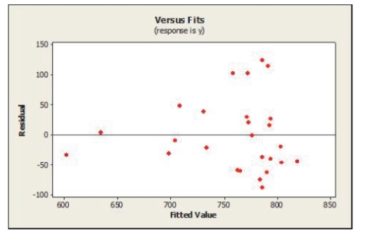
(Multiple Choice)
5.0/5 (37)
Filters
- Essay(0)
- Multiple Choice(0)
- Short Answer(0)
- True False(0)
- Matching(0)