A study was conducted to investigate variables associated with dropping out of high school. The following logistic regression model was obtained: Logit(YS1U1B1iS1U1B0) = 3.5 - 1.3XS1U1B11S1U1B0 + 2.3XS1U1B12S1U1B0. Y: 1 = dropped out of high school; 0 = did not drop out of high school; XS1U1B11S1U1B0: cumulative high school GPA obtained; XS1U1B12S1U1B0: 1 = retained in at least one grade; 0 = never retained in any grade. -If Mindy has a high school GPA of 3, and has never repeated a grade, which of the following predictions can be derived from the model?

A) Mindy has more than 50% probability of dropping out of high school. B) Mindy has less than 50% probability of dropping out of high school. C) Mindy has exactly 50% probability of dropping out of high school. D) Mindy will drop out of high school. E) Mindy will not drop out of high school. A) Mindy has more than 50% probability of dropping out of high school. B) Mindy has less than 50% probability of dropping out of high school. C) Mindy has exactly 50% probability of dropping out of high school. D) Mindy will drop out of high school. E) Mindy will not drop out of high school.

Complete the missing information for this table (Y is a dichotomous variable). $\begin{array}{ccc} \hline P(Y=1) & P(Y=0) & O d d s(Y=1) \\ \hline 0.10 & & \\ 0.25 & & \\ 0.40 & & \\ 0.20 & & \\ 0.90 & & \\ 0.75 & & \\ 0.60 & & \\ \hline \end{array}$

P(Y = 0) = 1 -P(Y = 1). Odds(Y = 1) = P(

A study was conducted to investigate variables associated with dropping out of high school. The following logistic regression model was obtained: Logit(YS1U1B1iS1U1B0) = 3.5 - 1.3XS1U1B11S1U1B0 + 2.3XS1U1B12S1U1B0. Y: 1 = dropped out of high school; 0 = did not drop out of high school; XS1U1B11S1U1B0: cumulative high school GPA obtained; XS1U1B12S1U1B0: 1 = retained in at least one grade; 0 = never retained in any grade. -What is being predicted in this model?

A) The mean difference in cumulative GPA between students who dropped out of high school and those who finished high school. B) The percentage of students who will drop out before graduating high school. C) The odds that a student will drop out of high school. D) The odds that a student had been retained in at least one grade if he dropped out of high school. A) The mean difference in cumulative GPA between students who dropped out of high school and those who finished high school. B) The percentage of students who will drop out before graduating high school. C) The odds that a student will drop out of high school. D) The odds that a student had been retained in at least one grade if he dropped out of high school.

A study was conducted to investigate variables associated with dropping out of high school. The following logistic regression model was obtained: Logit(YS1U1B1iS1U1B0) = 3.5 - 1.3XS1U1B11S1U1B0 + 2.3XS1U1B12S1U1B0. Y: 1 = dropped out of high school; 0 = did not drop out of high school; XS1U1B11S1U1B0: cumulative high school GPA obtained; XS1U1B12S1U1B0: 1 = retained in at least one grade; 0 = never retained in any grade. -Based on logistic regression, if a student has been retained in at least one grade, the chance that he/she will drop out of high school

A) increases. B) decreases. C) stays the same. D) is uncertain. A) increases. B) decreases. C) stays the same. D) is uncertain.

Exam 19: Logistic Regression

Complete the missing information for Table 1, using 0.50 as the cut value. Then complete the classification table (Table 2). Compute sensitivity, specificity, false positive rate, and false negative rate. Table 1. Observed group membership Predicted Probability Predicted group membership 1 0.88 1 0.72 0 0.62 1 0.49 0 0.34 1 0.40 1 0.60 0 0.21 0 0.05 1 0.57 Table 2. .00 1.00 Observed .00 1.00

Free

(Essay)

4.9/5

(41)

Question 1

Correct Answer:

Verified

Assuming 0.5 is the cut value, cases with predicted probabilities at .5 or above are predicted as 1 and predicted probabilities below .5 are predicted as 0. There are four cases with observed value 1 and predicted value 1. There are three cases with observed value 0 and predicted value 0. There is one case with observed value 0 yet predicted value 1 (false positive).
There are two cases with observed value 1 yet predicted value 0 (false negative).

Sensitivity = 4/(2+4) = 0.67 = 67%
Specificity = 3/(3+1) = 0.75 = 75%
False positive rate = 1/(3+1) = 0.25 -25%
False negative rate = 2/(2+4) = 0.33 = 33%

$\begin{array}{l}\text { Table } 1 .\\\begin{array}{ccc}\hline \begin{array}{c}\text { Observed group } \\\text { membership }\end{array} & \begin{array}{c}\text { Predicted } \\\text { Probability }\end{array} & \begin{array}{c}\text { Predicted group } \\\text { membership }\end{array} \\\hline 1 & 0.88 & 1 \\1 & 0.72 & 1 \\0 & 0.62 & 1 \\1 & 0.49 & 0 \\0 & 0.34 & 0 \\1 & 0.40 & 0 \\1 & 0.60 & 1 \\0 & 0.21 & 0 \\0 & 0.05 & 0 \\1 & 0.57 & 1 \\\hline\end{array}\end{array}$

$\begin{array}{l}\text { Table } 2 .\\\begin{array}{cccc}\hline & &&\underline { \text { Predicted }} \\& & .00 & &1.00 \\\hline{\text { Observed }} & .00 & 3&& 1\\& 1.00 &2& & 4\\\hline\end{array}\end{array}$

-What is the false negative rate?

Free

(Multiple Choice)

4.8/5

(27)

Question 2

Correct Answer:

Verified

You are given the following data, where X₁ (sex; male = 0, female =1; use 0 as the reference category) and X₂ (having at least one immediate family member who smokes; yes = 1, no = 0; use 0 as the reference category) are used to predict Y (being a smoker = 1 vs. being a nonsmoker = 0). ( $\alpha$ = .05) 0 0 1 0 0 0 0 1 1 0 1 1 1 0 0 1 0 0 1 0 1 1 0 0 1 1 1 1 1 0 Determine the following values based on simultaneous entry of independent variables: -2LL, constant, b₁, b₂, se(b₁), se(b₂), odds ratios, Wald₁, Wald₂.

Free

(Essay)

4.8/5

(33)

Question 3

Correct Answer:

Verified

-2LL = 10.688;
b₁_(Sex) = 1.792, b_2(Family) = 1.792, b_constant = -1.386;
se(b₁_(Sex)) = 1.571, se(b₂_(Family)) = 1.571;
odds ratio₁_(Sex) = 6.000, odds ratio₂₍_Family₎ = 6.000;
Wald₁_(Sex) = 1.301, Wald₂_(Family) = 1.301.

Procedure:
Create a data set with three variables: Sex (X₁), Family (X₂), and Smoke (Y). The data set should have 10 cases.
Follow the steps described in Question 2.
Use Smoke as the dependent variable, and Sex and Family as the covariates.

In step 3, move both Sex and Family into the Categorical Covariates box. Select Reference Category: First. Click Change.

Selected SPSS Output:
$\begin{array}{l}\text { Model Summary }\\\begin{array}{cccc}\hline \text { Step } & -2 \text { Log likelihood } & \text { Cox \& Snell } R \text { Square } & \text { Nagelkerke } R \text { Square } \\\hline 1 & 10.688^{\mathbf{a}} & .272 & .363 \\\hline\end{array}\end{array}$
$\begin{array}{l}\text { Hosmer and Lemeshow Test }\\\begin{array}{cccc}\hline \text { Step } & \text { Chi-square } & d f & \text { Sig. } \\\hline 1 & .451 & 2 & .798 \\\hline\end{array}\end{array}$
$\begin{array}{l}\text { Variables in the Equation }\\\hline\begin{array}{r}\underline { 95 \% \text { C.I. for } \mathrm{EXP}(\mathrm{B})}\\\begin{array}{cccccccccc}&&\text { B } & \text { S.E. } & \text { Wald } & d f & \text { Sig. } & \operatorname{Exp}(B)&\text { Lower }&\text { Upper } \\\hline & \operatorname{Sex}(1) & 1.792 & 1571 & 1.301 & 1 & .254 & 6.000 & .276 & 130.426 \\{\text { Step }} &\text { Family(1) } & 1.792 & 1571 & 1.301 & 1 & .254 & 6.000 & .276 & 130.426 \\1^{1}& \text { Constant } & -1.386 & 1.160 & 1.428 & 1 & .232 & .250 & & \\\hline\end{array}\end{array}\end{array}$
$\text { a. Variable(s) entered on step 1: Sex, Family. }$

Which one of the following can be used as an appropriate dependent variable for binary logistic regression?

(Multiple Choice)

4.7/5

(34)

Question 4

If a person is predicted to be a smoker, we would expect that

(Multiple Choice)

4.8/5

(30)

Question 5

-Aaron is studying smoking behavior and has coded "smoker" as "1" and "nonsmoker" as "0." The predictor is the number of family members who smoke. Which of the following is a correct interpretation of an odds ratio of +2?

(Multiple Choice)

4.8/5

(41)

Question 6

A study was conducted to investigate variables associated with dropping out of high school. The following logistic regression model was obtained: Logit(Y_i) = 3.5 - 1.3X₁ + 2.3X₂. Y: 1 = dropped out of high school; 0 = did not drop out of high school; X₁: cumulative high school GPA obtained; X₂: 1 = retained in at least one grade; 0 = never retained in any grade. -If Mindy has a high school GPA of 3, and has never repeated a grade, which of the following predictions can be derived from the model?

(Multiple Choice)

4.8/5

(34)

Question 7

Complete the missing information for this table (Y is a dichotomous variable). P(Y=1) P(Y=0) Odds(Y=1) 0.10 0.25 0.40 0.20 0.90 0.75 0.60

(Essay)

4.9/5

(35)

Question 8

A study was conducted to investigate variables associated with dropping out of high school. The following logistic regression model was obtained: Logit(Y_i) = 3.5 - 1.3X₁ + 2.3X₂. Y: 1 = dropped out of high school; 0 = did not drop out of high school; X₁: cumulative high school GPA obtained; X₂: 1 = retained in at least one grade; 0 = never retained in any grade. -What is being predicted in this model?

(Multiple Choice)

4.9/5

(40)

Question 9

-What is the false positive rate?

(Multiple Choice)

4.8/5

(37)

Question 10

The odds ratio is computed by which of the following?

(Multiple Choice)

4.8/5

(32)

Question 11

A study was conducted to investigate variables associated with dropping out of high school. The following logistic regression model was obtained: Logit(Y_i) = 3.5 - 1.3X₁ + 2.3X₂. Y: 1 = dropped out of high school; 0 = did not drop out of high school; X₁: cumulative high school GPA obtained; X₂: 1 = retained in at least one grade; 0 = never retained in any grade. -Based on logistic regression, if a student has been retained in at least one grade, the chance that he/she will drop out of high school

(Multiple Choice)

5.0/5

(30)

Question 12

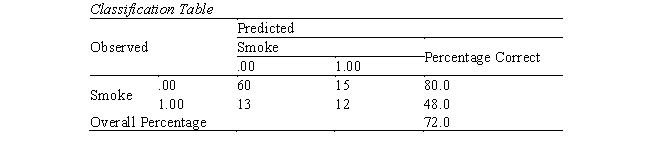
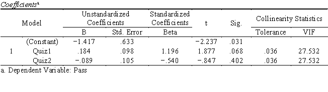
Professor Pruefung wanted to examine if performance in quizzes can predict whether a student will pass or fail the final exam. The independent variables are scores in two pop quizzes (Quiz1, Quiz2), and the dependent variable is a dichotomous variable (pass = 1 vs. fail = 0). Below is part of the output of the analysis. a. Professor Pruefung assumed that the better a student performed in the quizzes (a higher score indicates better performance), the higher the odds that he/she will pass the final exam. If that is the case, what are the expected signs for b₁ and b₂? Do the results confirm the expectation? b. Based on the tables, is there any indication of assumptions violation? If so, which assumption(s) has (have) been violated? c. What are the possible consequences of the assumption violation? $\text { Om nibus Tests of Model Coeffcients }$ Chi-square df Sig. Step Step 24.055 2 .000 1 Block 24.055 2 .000 Model 24.055 2 .000 $\text { Model Summary }$ Step -2 Cox \& Snell Nagelkerke likelihood R Square R Square 1 22.998 .452 .653 Variables in the Equation B S.E. Wald df Sig. Exp () Step 1 Quiz1 1.557 1.064 2.140 1 .143 4.745 Quiz2 -.535 1.023 .273 1 .601 .586 Constant -21.721 8.990 5.838 1 .016 .000 $Professor Pruefung wanted to examine if performance in quizzes can predict whether a student will pass or fail the final exam. The independent variables are scores in two pop quizzes (Quiz1, Quiz2), and the dependent variable is a dichotomous variable (pass = 1 vs. fail = 0). Below is part of the output of the analysis. a. Professor Pruefung assumed that the better a student performed in the quizzes (a higher score indicates better performance), the higher the odds that he/she will pass the final exam. If that is the case, what are the expected signs for b<sub>1</sub> and b<sub>2</sub>? Do the results confirm the expectation? b. Based on the tables, is there any indication of assumptions violation? If so, which assumption(s) has (have) been violated? c. What are the possible consequences of the assumption violation? \text { Om nibus Tests of Model Coeffcients } \begin{array}{ccccc} \hline & & \text { Chi-square } & d f & \text { Sig. } \\ \hline{\text { Step }} & \text { Step } & 24.055 & 2 & .000 \\ 1 & \text { Block } & 24.055 & 2 & .000 \\ & \text { Model } & 24.055 & 2 & .000 \end{array} \text { Model Summary } \begin{array}{cccc} \hline {\text { Step }} & {-2 \mathrm{Log}} & \text { Cox \& Snell} & \text {Nagelkerke } \\ & \text { likelihood } & R \text { Square } & R \text { Square } \\ \hline 1 & 22.998 & .452 & .653 \end{array} \begin{array}{l} \text { Variables in the Equation }\\ \begin{array}{llllllll} \hline & & \text { B } & \text { S.E. } & \text { Wald } & d f & \text { Sig. } & \operatorname{Exp}(\mathrm{B}) \\ \hline {\text { Step 1 }} & \text { Quiz1 } & 1.557 & 1.064 & 2.140 & 1 & .143 & 4.745 \\ & \text { Quiz2 } & -.535 & 1.023 & .273 & 1 & .601 & .586 \\ & \text { Constant } & -21.721 & 8.990 & 5.838 & 1 & .016 & .000 \\ \hline \end{array} \end{array}$

(Essay)

5.0/5

(37)

Question 13

You are given the following data, where X₁ (high school cumulative GPA) and X₂ (having repeated grade; 0 = never repeated any grade and 1 = have repeated at least one grade; use 0 as the reference category) are used to predict Y (dropping out of high school, "1," vs. graduating high school, "0"). ( $\alpha$ = .05) 2.50 1 0 2.60 0 0 2.75 0 0 1.33 1 1 3.00 1 0 3.42 0 0 2.70 1 1 2.33 1 1 1.75 0 1 2.80 0 0 Determine the following values based on simultaneous entry of the independent variables: -2LL, constant, b₁, b₂, se(b₁), se(b₂), odds ratios, Wald₁, Wald₂.

(Essay)

4.7/5

(36)

Question 14

Which one of the following can occur when the number of variables equals, or nearly equals, the number of cases in the data?

(Multiple Choice)

4.8/5

(36)

Question 15

Showing 1 - 15 of 15

-What is the false negative rate?

Which one of the following can be used as an appropriate dependent variable for binary logistic regression?

If a person is predicted to be a smoker, we would expect that

-Aaron is studying smoking behavior and has coded "smoker" as "1" and "nonsmoker" as "0." The predictor is the number of family members who smoke. Which of the following is a correct interpretation of an odds ratio of +2?

Complete the missing information for this table (Y is a dichotomous variable). P(Y=1) P(Y=0) Odds(Y=1) 0.10 0.25 0.40 0.20 0.90 0.75 0.60

-What is the false positive rate?

The odds ratio is computed by which of the following?

Which one of the following can occur when the number of variables equals, or nearly equals, the number of cases in the data?

Introduction

Data Representation

Univariate Population Parameters and Sample Statistics

The Normal Distribution and Standard Scores

Introduction to Probability and Sample Statistics

Introduction to Hypothesis Testing: Inferences About a Single Mean

Inferences About the Difference Between Two Means

Inferences About Proportions

Inferences About Variances

Bivariate Measures of Association

One-Factor Anova: Fixed-Effects Mode

Multiple Comparison Procedures

Factorial Anova: Fixed-Effects Mode

One Factor Fixed-Effects Ancova With Single Covariate

Random- and Mixed-Effects Analysis of Variance Models

Hierarchical and Randomized Block Analysis of Variance Models

Simple Linear Regression

Multiple Linear Regression

Mediation and Moderation

Filters