Question 1

In a multiple linear regression with three independent variables, X1, X2, and X3, which one of the following reflects an example of a semipartial correlation?

Accepted Answer

A)  The correlation between X1 and X2 and X3 where both X2 and X3 are removed from X1 and X2 
B)  The correlation between X1 and X2 where X3 is held constant 
C)  The correlation between X2 and X3 where X1 is partialed out 
D)  The correlation between X1 and X2 where X3 is removed from X2 only 
A)  The correlation between X1 and X2 and X3 where both X2 and X3 are removed from X1 and X2 
B)  The correlation between X1 and X2 where X3 is held constant 
C)  The correlation between X2 and X3 where X1 is partialed out 
D)  The correlation between X1 and X2 where X3 is removed from X2 only D

Question 2

The scatterplot of X and Y are shown as follows.
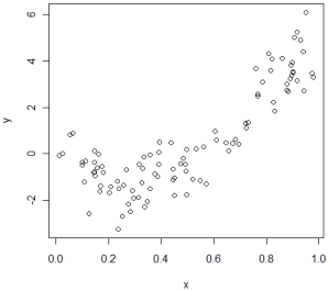  Based on the plot, which model is the most appropriate to use?

Accepted Answer

A)  Yi = b1Xi + a + ei. 
B)  Yi = b1Xi + b2Xi2 + a + ei. 
C)  Yi = b1Xi2 + a + ei. 
D)  Yi = b1Xi + b2Xi + b3Xi3 + a + ei. 
A)  Yi = b1Xi + a + ei. 
B)  Yi = b1Xi + b2Xi2 + a + ei. 
C)  Yi = b1Xi2 + a + ei. 
D)  Yi = b1Xi + b2Xi + b3Xi3 + a + ei. B

Question 3

You are given the following data, where X1 (attendance rate) and X2 (average SAT score) are to be used to predict Y (average score in graduation test). Each case represents one school.

$\begin{array}{|c|c|c|}
\hline Y & X_{\mathbf{1}} & X_{\mathbf{2}} \
\hline 78.4 & 93.4 & 1010 \
\hline 81.3 & 94.6 & 1020 \
\hline 81.3 & 95.4 & 1024 \
\hline 82.5 & 91.1 & 1136 \
\hline 77.8 & 91.6 & 952 \
\hline 84.5 & 94.2 & 1042 \
\hline 88.2 & 94.5 & 1106 \
\hline 88.7 & 93.4 & 1004 \
\hline 72.5 & 92.1 & 880 \
\hline 85.4 & 94.9 & 1124 \
\hline 82.9 & 94.3 & 1124 \
\hline 81.4 & 94.7 & 996 \
\hline
\end{array}$
 Determine the following values: intercept, b1, b2, SSres, SSreg, F, sres2, s(b1), s(b2), t1, t2.

Accepted Answer

Intercept = -36.536, b₁ = .869, b₂ = .036. SS_re_g = 120.957, SS_re_s = 103.365, F(2,9) = 5.266 (p = .031, reject at .05), s²_res = 11.485. s(b₁) = .764, s(b₂) = .014, t₁ = 1.138 (p = .285, fail to reject at .05), t₂ = 2.608 (p = .028, reject at .05). Procedure: Create a data set with three variables: Test (Y), Attend (X₁), and SAT (X₂). The data set should have 12 cases. 1) Go to Analyze$\rightarrow$ Regression $\rightarrow$ Linear. 2) Select Test to the Dependent list. Select Attend and SAT to the Independent(s) list. "3) Click OK. Selected SPSS Output: $\text { Model Summary }$ $\begin{array}{ccccc} \hline \text { Model } & R & R \text { Square } & \text { Adjusted } R \text { Square } & \text { Std. Error of the Estimate } \ \hline 1 & .734^{a} & .539 & .437 & 3.3890 \ \hline \end{array}$ $\text { a. Fredictors: (Constant), SAT, Attend }$ $\text { ANOVA }{ }^{\mathrm{b}}$ $\begin{array}{cccccc} \hline \text { Model } & \text { Sum of Squares } & d f & \text { Mean Square } & F & \text { Sig. } \ \hline \text { Regression } & \mathbf{1 2 0 . 9 5 7} & 2 & 60.479 & \mathbf{5 . 2 6 6} & \mathbf{. 0 3 1}^{\mathbf{a}} \ 1\text { Residual } & \mathbf{1 0 3 . 3 6 5} & 9 & \mathbf{1 1 . 4 8 5} & & \ \text { Total } & 224.323 & 11 & & &\ \hline \end{array}$ a. Fredictors: (Constant), SAT, Attend b. Dependent Variable: Test 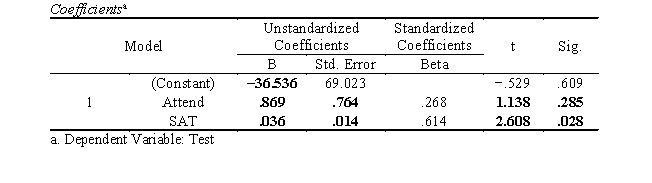Results: The results of the multiple linear regression suggest that a significant proportion of the total variation in graduation test scores was effectively predicted by attendance rate and SAT scores, F(2,9) = 5.266, p = .031. For Attend, the unstandardized partial slope (.869) and standardized partial slope (.268) are not statistically significantly different from 0 (t = 1.138, df = 9, p = .285). For SAT, the unstandardized partial slope (.036) and standardized partial slope (.614) are statistically significantly different from 0 (t = 2.608, df = 9, p = .028); with every point increase in SAT score, the graduation test score is expected to increase by .036 controlling for attendance rate. Multiple R² indicates that 53.9% of the variation in graduation test scores was predicted by attendance rate and SAT score. This suggests a large effect size. The intercept was -36.536, which is not statistically significantly different from 0 at .05 level (t = -.529, df = 9, p = .609)."

Question 4

You are given the following data, where X1 (Pretest score) and X2 (Hours spent in the program) are used to predict Y (Posttest score):

$\begin{array}{ccc}
\hline \boldsymbol{Y} & \boldsymbol{X}_{\mathbf{1}} & \boldsymbol{X}_{\mathbf{2}} \
\hline 65 & 60 & 7.5 \
82 & 62 & 9.0 \
94 & 75 & 8.5 \
80 & 78 & 7.0 \
87 & 65 & 10.0 \
66 & 60 & 8.0 \
\hline
\end{array}$
 Determine the following values: intercept, b1, b2, SSres, SSreg, F, sres2, s(b1), s(b2), t1, t2.

Accepted Answer

Intercept = -70.662, b₁ = 1.2

Question 5

Complete the missing information for this regression model (df = 25).

Accepted Answer

t₁ = b₁/s(b_1<

Question 6

For the regression model, Yi = b1X1i + b2X2i + a + ei, consider the following two situations:
Situation 1: rY1 = ?0.5 rY2 = 0.8 r12 = 0.1
Situation 2: rY1 = 0.2 rY2 = 0.8 r12 = 0.1
In which of the two situations will R2 be larger?

Accepted Answer

A)  Situation 1. 
B)  Situation 2. 
C)  R2 will be the same in both situations. 
D)  Uncertain. 
A)  Situation 1. 
B)  Situation 2. 
C)  R2 will be the same in both situations. 
D)  Uncertain.

Question 7

Which of the following situations will result in the best prediction in multiple regression analysis?

Accepted Answer

A)  rY1 = 0.1 rY2 = 0.4 r12 = 0.1 
B)  rY1 = 0.1 rY2 = 0.4 r12 = 0.8 
C)  rY1 = 0.6 rY2 = 0.4 r12 = 0.1 
D)  rY1 = 0.6 rY2 = 0.4 r12 = 0.8 
A)  rY1 = 0.1 rY2 = 0.4 r12 = 0.1 
B)  rY1 = 0.1 rY2 = 0.4 r12 = 0.8 
C)  rY1 = 0.6 rY2 = 0.4 r12 = 0.1 
D)  rY1 = 0.6 rY2 = 0.4 r12 = 0.8

Question 8

Which one of the following reflects variables appropriate for a multiple linear regression model?

Accepted Answer

A)  One categorical dependent variable and one continuous independent variable 
B)  One continuous dependent variable and one continuous or categorical independent variable 
C)  One continuous dependent variable and two or more continuous independent variables 
D)  Two or more continuous dependent variables and one continuous or categorical independent variable 
A)  One categorical dependent variable and one continuous independent variable 
B)  One continuous dependent variable and one continuous or categorical independent variable 
C)  One continuous dependent variable and two or more continuous independent variables 
D)  Two or more continuous dependent variables and one continuous or categorical independent variable

Question 9

Partial correlations allow for which one of the following in multiple linear regression?

Accepted Answer

A)  Design control 
B)  Experiential control 
C)  Experimental control 
D)  Statistical control 
A)  Design control 
B)  Experiential control 
C)  Experimental control 
D)  Statistical control

Question 10

A researcher would like to predict GPA from a set of three predictor variables for a sample of 34 college students. Multiple linear regression analysis was utilized. Complete the following summary table 
($\alpha$= .05) for the test of significance of the overall regression model:

Accepted Answer

There are three independent variables, s

In a multiple linear regression with three independent variables, X₁, X₂, and X₃, which one of the following reflects an example of a semipartial correlation?

The scatterplot of X and Y are shown as follows. Based on the plot, which model is the most appropriate to use?

Complete the missing information for this regression model (df = 25).

For the regression model, Y_i = b₁X₁_i + b₂X₂_i + a + e_i, consider the following two situations: Situation 1: r_Y₁ = ?0.5 r_Y₂ = 0.8 r₁₂ = 0.1 Situation 2: r_Y₁ = 0.2 r_Y₂ = 0.8 r₁₂ = 0.1 In which of the two situations will R² be larger?

Which of the following situations will result in the best prediction in multiple regression analysis?

Which one of the following reflects variables appropriate for a multiple linear regression model?

Partial correlations allow for which one of the following in multiple linear regression?

Introduction

Data Representation

Univariate Population Parameters and Sample Statistics

The Normal Distribution and Standard Scores

Introduction to Probability and Sample Statistics

Introduction to Hypothesis Testing: Inferences About a Single Mean

Inferences About the Difference Between Two Means

Inferences About Proportions

Inferences About Variances

Bivariate Measures of Association

One-Factor Anova: Fixed-Effects Mode

Multiple Comparison Procedures

Factorial Anova: Fixed-Effects Mode

One Factor Fixed-Effects Ancova With Single Covariate

Random- and Mixed-Effects Analysis of Variance Models

Hierarchical and Randomized Block Analysis of Variance Models

Simple Linear Regression

Logistic Regression

Mediation and Moderation

Filters

Exam 18: Multiple Linear Regression

In a multiple linear regression with three independent variables, X1, X2, and X3, which one of the following reflects an example of a semipartial correlation?

The scatterplot of X and Y are shown as follows. Based on the plot, which model is the most appropriate to use?

You are given the following data, where X1 (Pretest score) and X2 (Hours spent in the program) are used to predict Y (Posttest score): 65 60 7.5 82 62 9.0 94 75 8.5 80 78 7.0 87 65 10.0 66 60 8.0 Determine the following values: intercept, b1, b2, SSres, SSreg, F, sres2, s(b1), s(b2), t1, t2.

Complete the missing information for this regression model (df = 25).

For the regression model, Yi = b1X1i + b2X2i + a + ei, consider the following two situations: Situation 1: rY1 = ?0.5 rY2 = 0.8 r12 = 0.1 Situation 2: rY1 = 0.2 rY2 = 0.8 r12 = 0.1 In which of the two situations will R2 be larger?

Which of the following situations will result in the best prediction in multiple regression analysis?

Which one of the following reflects variables appropriate for a multiple linear regression model?

Partial correlations allow for which one of the following in multiple linear regression?

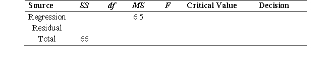
A researcher would like to predict GPA from a set of three predictor variables for a sample of 34 college students. Multiple linear regression analysis was utilized. Complete the following summary table ( α\alphaα = .05) for the test of significance of the overall regression model:

Introduction

Data Representation

Univariate Population Parameters and Sample Statistics

The Normal Distribution and Standard Scores

Introduction to Probability and Sample Statistics

Introduction to Hypothesis Testing: Inferences About a Single Mean

Inferences About the Difference Between Two Means

Inferences About Proportions

Inferences About Variances

Bivariate Measures of Association

One-Factor Anova: Fixed-Effects Mode

Multiple Comparison Procedures

Factorial Anova: Fixed-Effects Mode

One Factor Fixed-Effects Ancova With Single Covariate

Random- and Mixed-Effects Analysis of Variance Models

Hierarchical and Randomized Block Analysis of Variance Models

Simple Linear Regression

Logistic Regression

Mediation and Moderation

Filters

In a multiple linear regression with three independent variables, X₁, X₂, and X₃, which one of the following reflects an example of a semipartial correlation?

For the regression model, Y_i = b₁X₁_i + b₂X₂_i + a + e_i, consider the following two situations: Situation 1: r_Y₁ = ?0.5 r_Y₂ = 0.8 r₁₂ = 0.1 Situation 2: r_Y₁ = 0.2 r_Y₂ = 0.8 r₁₂ = 0.1 In which of the two situations will R² be larger?