Exam 8: Elaboration of Tabular Data and the Nature of Causation
You are wondering whether the relationship between being a minority and arrest remains statistically significant when taking the seriousness of the traffic violation into consideration. Compute chi square and phi. Compute chi square (minority, arrest) holding severity of traffic violation constant.
a. Organize your data in tables and then identify the IVs and DVs.
b. State your null and alternative hypotheses.
c. Compute the degrees of freedom for each test.
d. State your decision rule using the chi square table.
e. Compute chi square (χ2).
f. Make your decision and interpret your findings for each test.
a. (IV = seriousness; DV = arrest) and (0 = minor; 1 = serious).
b. H0: There is no statistically significant difference between severity of the traffic violation and arrests after a traffic stop.
H1: There is a statistically significant difference severity of the traffic violation and arrests after a traffic stop.
c. df = (c - 1) × (r - 1) = 1.
d. You reject the null hypothesis if χ2 is greater than ±3.841.
e.
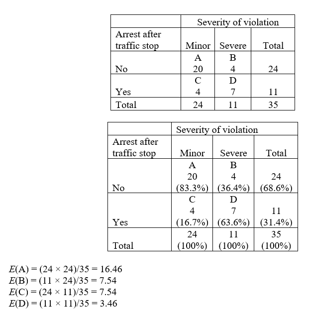
f. You reject the null hypothesis (alpha 0.05) because χ (7.7072) exceeds 3.841, meaning that there is a statistically significant moderate (phi = 0.4693) relationship between the severity of a traffic violation and arrest (χ2(1) = 7.7072, p < 0.05). Whereas 63.6% of individuals stopped for a severe traffic violation were subsequently arrested, only 16.7% of individuals stopped for a minor traffic violation were. The value of chi square also indicates that severity of the traffic violation has a greater influence on an arrest decision than being a minority driver.
Arrest × Race (minor violation)
E(A) = (16 × 20)/24 = 13.33
E(B) = (8 × 20)/24 = 6.67
E(C) = (16× 4)/24 = 2.67
E(D) = (8 × 4)/24 = 1.33
χ2(1) = 3.7688, p > 0.05, not significant.
Arrest× Race (severe violation)
E(A) = (7 × 4)/11 = 2.55
E(B) = (4 × 4)/11 = 1.45
E(C) = (7 × 7)/11 = 4.45
E(D) = (4 × 7)/11 = 2.55
χ2(1) = 3.5715, p > 0.05, not significant.
When we take the seriousness of the traffic violation into account, the relationship between being a minority and arrest disappears, with χ2 values not reaching the critical value of 3.841. Thus, the hypothesis that minorities have a higher overall arrest rate after a traffic stop is not supported with these data. Recall that the scenarios are purely hypothetical.
Indicate whether in the following examples the IV is necessary, sufficient, both, or neither.
a. The willingness to change is a _____________ cause of desistance.
b. Driving under the influence of alcohol is a ______________ cause for arrest.
c. Being born in the United States is a ________________ cause for U.S. citizenship.
d. Being convicted for an offense is a ___________________ cause for a criminal record.
a. Necessary.
b. Sufficient.
c. Sufficient.
d. Necessary and sufficient.
To determine whether one variable (IV) is predicting another variable (DV) to a certain degree, statisticians make use of multivariate analyses and thus are introducing other variables (IVs) as so-called ________________ variables.
Control variables.
What are the requirements to establish causality? Indicate the meaning of the terms. Also provide an example in which the requirement is absent.
a. __________________________________
b. __________________________________
c. __________________________________
Assume you are interested to find what variables influence the decision-making process of a police officer to arrest an individual after being stopped because of a traffic violation (0 = no arrest; 1 = arrest). First, you question whether race (0 = nonminority; 1 = minority) could have some influence on an officer's decision to make an arrest. Then, you ask whether seriousness of the traffic offense influences the outcome of arrest (0 = minor; 1= severe). The hypothetical data (n = 35) are presented in the table below. You set your alpha level at 0.05.
Case Arrest Race Seriousness Case Arrest Race Seriousness 1 1 0 1 19 0 0 0 2 0 0 0 20 0 0 0 3 0 0 0 21 1 0 1 4 1 1 0 22 0 1 0 5 0 1 0 23 0 0 0 6 1 1 1 24 0 0 1 7 0 0 0 25 1 1 1 8 0 0 1 26 1 0 0 9 0 1 0 27 1 1 1 10 0 0 0 28 0 0 0 11 1 1 1 29 0 0 0 12 0 0 0 30 0 1 0 13 0 0 0 31 0 0 1 14 1 1 0 32 1 1 0 15 1 0 1 33 0 0 0 16 0 0 0 35 0 0 0 17 0 0 0 35 0 0 1 18 0 1 0
a. Organize your data in a table and then identify the IV and DV.
b. State your null and alternative hypotheses.
c. Compute the degrees of freedom.
d. State your decision rule using the chi square table.
e. Compute chi square (χ2).
f. Make your decision and interpret your findings.
Filters
- Essay(0)
- Multiple Choice(0)
- Short Answer(0)
- True False(0)
- Matching(0)