Exam 3: Introduction to Linear Programming
The Weigelt Corporation has three branch plants with excess production capacity.Fortunately,the corporation has a new product ready to begin production,and all three plants have this capability,so some of the excess capacity can be used in this way.This product can be made in three sizes--large,medium,and small--that yield a net unit profit of $420,$360,and $300,respectively.Plants 1,2,and 3 have the excess capacity to produce 750,900,and 450 units per day of this product,respectively,regardless of the size or combination of sizes involved.The amount of available in-process storage space also imposes a limitation on the production rates of the new product.Plants 1,2,and 3 have 13,000,12,000,and 5,000 square feet,respectively,of in-process storage space available for a day's production of this product.Each unit of the large,medium,and small sizes produced per day requires 20,15,and 12 square feet,respectively.Sales forecasts indicate that if available,900,1,200,and 750 units of the large,medium,and small sizes,respectively,would be sold per day.At each plant,some employees will need to be laid off unless most of the plant's excess production capacity can be used to produce the new product.To avoid layoffs if possible,management has decided that the plants should use the same percentage of their excess capacity to produce the new product.Management wishes to know how much of each of the sizes should be produced by each of the plants to maximize profit.Formulate a linear programming model for this problem.
The decision variables can be denoted and defined as follows: xP1L = number of large units produced per day at Plant 1,xP1M = number of medium units produced per day at Plant 1,xP1S = number of small units produced per day at Plant 1,xP2L = number of large units produced per day at Plant 2,xP2M = number of medium units produced per day at Plant 2,xP2S = number of small units produced per day at Plant 2,xP3L = number of large units produced per day at Plant 3,xP3M = number of medium units produced per day at Plant 3,xP3S = number of small units produced per day at Plant 3.Also letting P (or Z)denote the total net profit per day,the linear programming model for this problem is Maximize P = 420 xP1L + 360 xP1M + 300 xP1S + 420 xP2L + 360 xP2M + 300 xP2S + 420 xP3L + 360 xP3M + 300 xP3S,subject to xP1L + xP1M + xP1S 750 xP2L + xP2M + xP2S 900 xP3L + xP3M + xP3S 450 20 xP1L + 15 xP1M + 12 xP1S 13000 20 xP2L + 15 xP2M + 12 xP2S 12000 20 xP3L + 15 xP3M + 12 xP3S 5000 xP1L + xP2L + xP3L 900 xP1M + xP2M + xP3M 1200 xP1S + xP2S + xP3S 750  ( xP1L + xP1M + xP1S )-
  ( xP2L + xP2M + xP2S )= 0
  ( xP1L + xP1M + xP1S )-
  ( xP3L + xP3M + xP3S )= 0 and xP1L 0,xP1M 0,xP1S 0,xP2L 0,xP2M 0,xP2S 0,xP3L 0,xP3M 0,xP3S 0.The above set of equality constraints also can include the following constraint:
  = 0.However,any one of the three equality constraints is redundant,so any one (say,this one)can be deleted.
The kitchen manager for Sing Sing Prison is trying to decide what to feed its prisoners.She would like to offer some combination of milk,beans,and oranges.The goal is to minimize cost,subject to meeting the minimum nutritional requirements imposed by law.The cost and nutritional content of each food,along with the minimum nutritional requirements,are shown below.What diet should be fed to each prisoner?  (a)Formulate and solve a linear programming model for this problem in a spreadsheet.(b)Formulate this same model algebraically.
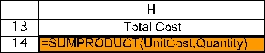
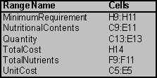
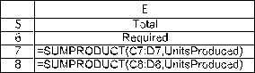
(a)This is a cost-benefit-trade-off problem.The activities are the quantities of food to feed each prisoner and the required benefits are the minimum nutritional requirements.We will start to build a spreadsheet by entering the data.The data for this problem are the nutrient content of each food,the minimum daily requirement for each nutrient,and the cost of each food.The data in the spreadsheet would be entered as displayed below,where range names of UnitCost (C5:E5),NutritionalContents (C9:E11),and MinimumRequirement (H9:H11)are assigned to the corresponding data cells. 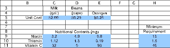 The decisions to be made in this problem are how much of each food type should be fed to each prisoner.Therefore,we add three changing cells in C13:E13,with range name Quantity.The values in Quantity (C13:E13)will eventually be determined by Solver.For now,an arbitrary value of 1 is entered for each food type.The goal is to minimize the total cost per prisoner.Thus,the objective cell should calculate this cost: Total Cost = ($2)(gallons of milk)+ ($0.20)(cups of beans)+ ($0.25)(number of oranges)or Total Cost = SUMPRODUCT(UnitCost,Quantity).This formula is entered into cell H14.
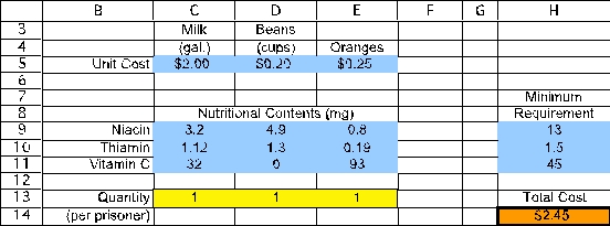
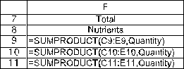
 The functional constraints in this problem involve the minimum daily requirement of each nutrient.Given the amount of food fed each prisoner (the changing cells in C13:E13),we calculate the total resources used in F9:F11.For niacin,this will be =SUMPRODUCT(C9:E9,$C$13:$E$13).Using an absolute reference for the acres planted,this formula can be copied into cells F10-F11 to calculate the thiamin and vitamin C.The benefit achieved (total of each nutrient)must be >= the minimum needed (H9:H11),as indicated by the >= in G9:G11.
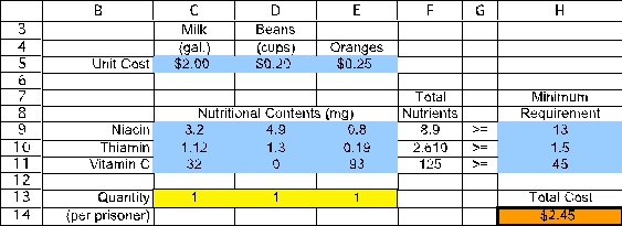
 The Solver information and solved spreadsheet are shown below.
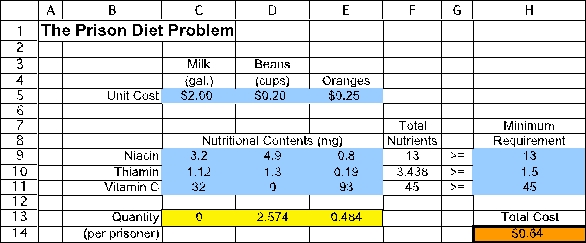
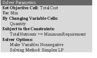

 Thus,each prisoner should be fed a daily average of 2.574 cups of beans and 0.484 oranges for a total cost of $0.64.(b)To build an algebraic model for this problem,start by defining the decision variables.In this case,the three decisions are how many gallons of milk,cups of beans,and how many oranges to feed each prisoner.These variables are defined below: Let M = gallons of milk fed to each prisoner,B = cups of beans fed to each prisoner,O = number of oranges fed to each prisoner.Next determine the goal of the problem.In this case,the goal is to meet the nutritional requirements at the lowest possible cost.Each gallon of milk costs $2,each cup of beans costs $0.20,and each orange costs $0.25.The objective function is therefore Minimize Total Cost = $2.00M + $0.20B + $0.25O.The nutritional requirements include minimum requirements for niacin,thiamin,and vitamin C.The data for the nutritional contents of each type of food can be used to calculate the total level of each nutrient achieved as a function of the decision variables.The total nutrients need to be greater than or equal to the minimum requirement.These constraints are therefore as follows: Niacin: 3.2M + 4.9B + 0.8O ≥ 13mg,Thiamin: 1.12M + 1.3B + 0.19O ≥ 1.5mg,Vitamin C: 32M + 93O ≥ 45mg.After adding nonnegativity constraints,the complete algebraic formulation is given below: Let M = gallons of milk fed to each prisoner,B = cups of beans fed to each prisoner,O = number of oranges fed to each prisoner.Minimize Total Cost = $2.00M + $0.20B + $0.25O.subject to Niacin: 3.2M + 4.9B + 0.8O ≥ 13mg,Thiamin: 1.12M + 1.3B + 0.19O ≥ 1.5mg,Vitamin C: 32M + 93O ≥ 45mg.and M ≥ 0,B ≥ 0,O ≥ 0.
Back Savers is a company that produces backpacks primarily for students.They are considering offering some combination of two different models-the Collegiate and the Mini.Both are made out of the same rip-resistant nylon fabric.Back Savers has a long-term contract with a supplier of the nylon and receives a 5000 square-foot shipment of the material each week.Each Collegiate requires 3 square feet while each Mini requires 2 square feet.The sales forecasts indicate that at most 1000 Collegiates and 1200 Minis can be sold per week.Each Collegiate requires 45 minutes of labor to produce and generates a unit profit of $32.Each Mini requires 40 minutes of labor and generates a unit profit of $24.Back Savers has 35 laborers that each provides 40 hours of labor per week.Management wishes to know what quantity of each type of backpack to produce per week.(a)Formulate and solve a linear programming model for this problem on a spreadsheet.(b)Formulate this same model algebraically.(c)Use the graphical method by hand to solve this model.
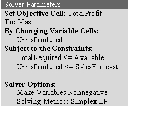
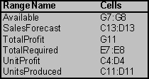
(a)To build a spreadsheet model for this problem,start by entering the data.The data for this problem are the unit profit of each type of backpack,the resource requirements (square feet of nylon and labor hours required),the availability of each resource,5400 square feet of nylon and (35 laborers)(40 hours/laborer)= 1400 labor hours,and the sales forecast for each type of backpack (1000 Collegiates and 1200 Minis).In order to keep the units consistent in row 8 (hours),the labor required for each backpack (in cells C8 and D8)are converted from minutes to hours (0.75 hours = 45 minutes,0.667 hours = 40 minutes).The range names UnitProfit (C4:D4),Available (G7:G8),and SalesForecast (C13:D13)are added for these data. 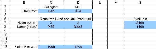 The decision to be made in this problem is how many of each type of backpack to make.Therefore,we add two changing cells with range name UnitsProduced (C11:D11).The values in CallsPlaced will eventually be determined by the Solver.For now,arbitrary values of 10 and 10 are entered.
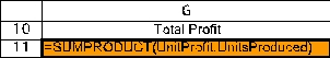
 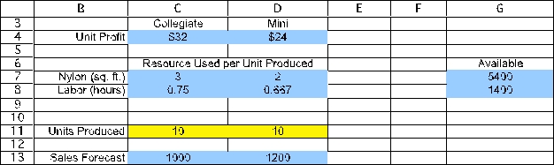 The goal is to produce backpacks so as to achieve the highest total profit.Thus,the objective cell should calculate the total profit,where the objective will be to maximize this objective cell.In this case,the total profit will be Total Profit = ($32)(# of Collegiates)+ ($24)(# of Minis)or Total Cost = SUMPRODUCT(UnitProfit,UnitsProduced).This formula is entered into cell G11 and given a range name of TotalProfit.With 10 Collegiates and 10 Minis produced,the total profit would be ($32)(10)+ ($24)(10)= $560.
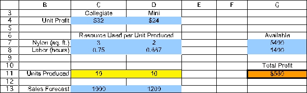
 The first set of constraints in this problem involve the limited available resources (nylon and labor hours).Given the number of units produced (UnitsProduced in C11:D11),we calculate the total resources required.For nylon,this will be =SUMPRODUCT(C7:D7,UnitsProduced)in cell E7.By using a range name or an absolute reference for the units produced,this formula can be copied into cell E8 to calculate the labor hours required.The total resources used (TotalResources in E7:E8)must be <= Available (in cells G7:G8),as indicated by the <= in F7:F8.
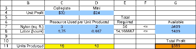
 The final constraint is that it does not make sense to produce more backpacks than can be sold (as predicted by the sales forecast).Therefore UnitsProduced (C11:D11)should be less-than-or-equal-to the SalesForecast (C13:D13),as indicated by the <= in C12:D12
 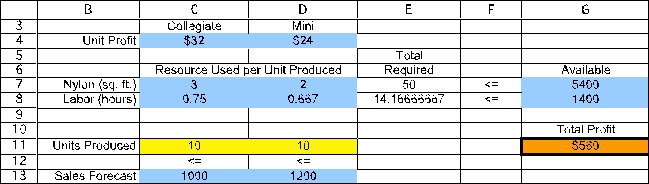 The Solver information and solved spreadsheet are shown below.
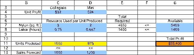

 Thus,they should produce 1000 Collegiates and 975 Minis to achieve the maximum total profit of $55,400.(b)To build an algebraic model for this problem,start by defining the decision variables.In this case,the two decisions are how many Collegiates to produce and how many Minis to produce.These variables are defined below: Let C = Number of Collegiates to produce,M = Number of Minis to produce.Next determine the goal of the problem.In this case,the goal is to produce the number of each type of backpack to achieve the highest possible total profit.Each Collegiate yields a unit profit of $32 while each Mini yields a unit profit of $24.The objective function is therefore Maximize Total Profit = $32C + $24M.The first set of constraints in this problem involve the limited resources (nylon and labor hours).Given the number of backpacks produced,C and M,and the required nylon and labor hours for each,the total resources used can be calculated.These total resources used need to be less than or equal to the amount available.Since the labor available is in units of hours,the labor required for each backpack needs to be in units of hours (3/4 hour and 2/3 hour)rather than minutes (45 minutes and 40 minutes).These constraints are as follows: Nylon: 3C + 2M ≤ 5400 square feet,Labor Hours: (3/4)C + (2/3)M ≤ 1400 hours.The final constraint is that they should not produce more of each backpack than the sales forecast.Therefore,Sales Forecast: C ≤ 1000 M ≤ 1200.After adding nonnegativity constraints,the complete algebraic formulation is given below: Let C = Number of Collegiates to produce,M = Number of Minis to produce.Maximize Total Profit = $32C + $24M,subject to Nylon: 3C + 2M ≤ 5400 square feet,Labor Hours: (3/4)C + (2/3)M ≤ 1400 hours,Sales Forecast: C ≤ 1000 M ≤ 1200.and C ≥ 0,M ≥ 0.(c)Start by plotting a graph with Collegiates (C)on the horizontal axis and Minis (M)on the vertical axis,as shown below.
 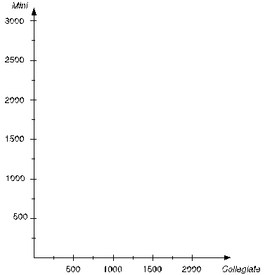 Next,the four constraint boundary lines (where the left-hand-side of the constraint exactly equals the right-hand-side)need to be plotted.The easiest way to do this is by determining where these lines intercepts the two axes.For the Nylon constraint boundary line (3C + 2M = 5400),setting M = 0 yields a C-intercept of 1800 while setting C = 0 yields an M-intercept of 2700.For the Labor constraint boundary line ((3/4)C + (2/3)M = 1400),setting M = 0 yields a C-intercept of 1866.67 while setting C = 0 yields an M-intercept of 2100.The sales forecast constraints are a horizontal line at M = 1200 and a vertical line at C = 1000.These constraint boundary lines are plotted below.
 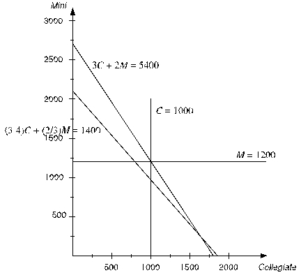 A feasible solution must be below and/or to the left of all four of these constraints while being above the Collegiate axis (since C ≥ 0)and to the right of the Mini axis (since M ≥ 0).This yields the feasible region shown below.
 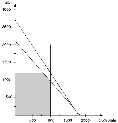 To find the optimal solution,an objective function line is plotted by setting the objective function equal to a value.For example,the objective function line when the value of the objective function is $48,000 is plotted as a dashed line below.
 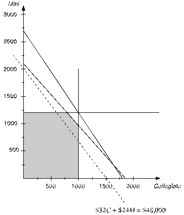 All objective function lines will be parallel to this one.To find the feasible solution that maximizes profit,slide this line out as far as possible while still touching the feasible region.This occurs when the profit is $55,400,and the objective function line intersect the feasible region at the single point with (C,M)= (1000,975)as shown below.
 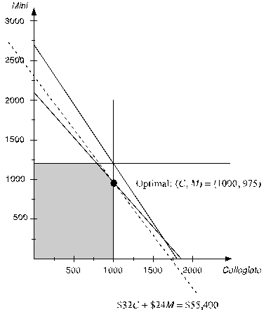 Therefore,the optimal solution is to produce 1000 Collegiates and 975 Minis,yielding a total profit of $55,400.
Comfortable Hands is a company which features a product line of winter gloves for the entire family - men,women,and children.They are trying to decide what mix of these three types of gloves to produce.Comfortable Hands' manufacturing labor force is unionized.Each full-time employee works a 40-hour week.In addition,by union contract,the number of full-time employees can never drop below 20.Nonunion,part-time workers can also be hired with the following union-imposed restrictions: (1)each part-time worker works 20 hours per week,and (2)there must be at least 2 full-time employees for each part-time employee.All three types of gloves are made out of the same 100% genuine cowhide leather.Comfortable Hands has a long term contract with a supplier of the leather,and receives a 5,000 square feet shipment of the material each week.The material requirements and labor requirements,along with the gross profit per glove sold (not considering labor costs)is given in the following table.  Each full-time employee earns $13 per hour,while each part-time employee earns $10 per hour.Management wishes to know what mix of each of the three types of gloves to produce per week,as well as how many full-time and how many part-time workers to employ.They would like to maximize their net profit - their gross profit from sales minus their labor costs.Formulate a linear programming model for this problem.
Dwight and Hattie have run the family farm for over thirty years.They are currently planning the mix of crops to plant on their 120-acre farm for the upcoming season.The table below gives the labor hours and fertilizer required per acre,as well as the total expected profit per acre for each of the potential crops under consideration.Dwight,Hattie,and their children can work at most 6,500 total hours during the upcoming season.They have 200 tons of fertilizer available.What mix of crops should be planted to maximize the family's total profit?  (a)Formulate and solve a linear programming model for this problem in a spreadsheet.(b)Formulate this same model algebraically.
Cool Power produces air conditioning units for large commercial properties.Due to the low cost and efficiency of its products,the company has been growing from year to year.Also,due to seasonality in construction and weather conditions,production requirements vary from month to month.Cool Power currently has 10 fully trained employees working in manufacturing.Each trained employee can work 160 hours per month and is paid a monthly wage of $4000.New trainees can be hired at the beginning of any month.Due to their lack of initial skills and required training,a new trainee only provides 100 hours of useful labor in their first month,but are still paid a full monthly wage of $4000.Furthermore,because of required interviewing and training,there is a $2500 hiring cost for each employee hired.After one month,a trainee is considered fully trained.An employee can be fired at the beginning of any month,but must be paid two weeks of severance pay ($2000).Over the next 12 months,Cool Power forecasts the labor requirements shown in the table below.Since management anticipates higher requirements next year,Cool Power would like to end the year with at least 12 fully trained employees.How many trainees should be hired and/or workers fired in each month to meet the labor requirements at the minimum possible cost? Formulate and solve a linear programming spreadsheet model. 
The marketing group for a cell phone manufacturer plans to conduct a telephone survey to determine consumer attitudes toward a new cell phone that is currently under development.In order to have a sufficient sample size to conduct the analysis,they need to contact at least 100 young males (under age 40),150 older males (over age 40),120 young females (under age 40),and 200 older females (over age 40).It costs $1 to make a daytime phone call and $1.50 to make an evening phone call (due to higher labor costs).This cost is incurred whether or not anyone answers the phone.The table below shows the likelihood of a given customer type answering each phone call.Assume the survey is conducted with whoever first answers the phone.Also,because of limited evening staffing,at most one-third of phone calls placed can be evening phone calls.How should the marketing group conduct the telephone survey so as to meet the sample size requirements at the lowest possible cost?  (a)Formulate and solve a linear programming model for this problem on a spreadsheet.(b)Formulate this same model algebraically.
Surfs Up produces high-end surfboards.A challenge faced by Surfs Up is that their demand is highly seasonal.Demand exceeds production capacity during the warm summer months,but is very low in the winter months.To meet the high demand during the summer,Surfs Up typically produces more surfboards than are needed in the winter months and then carries inventory into the summer months.Their production facility can produce at most 50 boards per month using regular labor at a cost of $125 each.Up to 10 additional boards can be produced by utilizing overtime labor at a cost of $135 each.The boards are sold for $200.Because of storage cost and the opportunity cost of capital,each board held in inventory from one month to the next incurs a cost of $5 per board.Since demand is uncertain,Surfs Up would like to maintain an ending inventory (safety stock)of at least 10 boards during the warm months (May-September)and at least 5 boards during the other months (October-April).It is now the start of January and Surfs Up has 5 boards in inventory.The forecast of demand over the next 12 months is shown in the table below.Formulate and solve a linear programming model in a spreadsheet to determine how many surfboards should be produced each month to maximize total profit. 
Slim-Down Manufacturing makes a line of nutritionally complete,weight-reduction beverages.One of their products is a strawberry shake which is designed to be a complete meal.The strawberry shake consists of several ingredients.Some information about each of these ingredients is given below.  The nutritional requirements are as follows.The beverage must total between 380 and 420 calories (inclusive).No more than 20% of the total calories should come from fat.There must be at least 50 milligrams (mg)of vitamin content.For taste reasons,there must be at least two tablespoons (tbsp)of strawberry flavoring for each tbsp of artificial sweetener.Finally,to maintain proper thickness,there must be exactly 15 mg of thickeners in the beverage.Management would like to select the quantity of each ingredient for the beverage which would minimize cost while meeting the above requirements.Formulate a linear programming model for this problem.
Filters
- Essay(0)
- Multiple Choice(0)
- Short Answer(0)
- True False(0)
- Matching(0)