Exam 12: Simple Linear Regression

The coefficient of determination represents the ratio of SSR to SST.

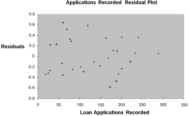
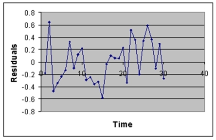
Instruction 12-12 The manager of the purchasing department of a large savings and loan organization would like to develop a model to predict the amount of time (measured in hours)it takes to record a loan application.Data are collected from a sample of 30 days,and the number of applications recorded and completion time in hours is recorded.Below is the regression output: Regression Statistics Multiple R 0.9447 R Square 0.8924 Adjusted R 0.8886 Square Standard 0.3342 Error Observations 30 ANOVA df SS MS F Significance F Regression 1 25.9438 25.9438 232.2200 4.3946-15 Residual 28 3.1282 0.1117 Total 29 29.072 Coefficients Standard Error t Stat P-value Lower 95\% Upper 95\% Intercept 0.4024 0.1236 3.2559 0.0030 0.1492 0.6555 Applications 0.0126 0.0008 15.2388 4.3946-15 0.0109 0.0143 Recorded Note: 4.3946E-15 is 4.3946 x 10^-15. -Referring to Instruction 12-12,there is no evidence of positive autocorrelation if the Durbin-Watson test statistic is found to be 1.78.

Instruction 12-4 The managers of a brokerage firm are interested in finding out if the number of new customers a broker brings into the firm affects the sales generated by the broker.They sample 12 brokers and determine the number of new customers they have enrolled in the last year and their sales amounts in thousands of dollars.These data are presented in the table that follows. Broker Clients Sales 1 27 52 2 11 37 3 42 64 4 33 55 5 15 29 6 15 34 7 25 58 8 36 59 9 28 44 10 30 48 11 17 31 12 22 38 -Referring to Instruction 12-4,the managers of the brokerage firm wanted to test the hypothesis that the number of new customers brought in had a positive impact on the amount of sales generated.At a level of significance of 0.01,the null hypothesis should be ________ (accepted or rejected).

Instruction 12-11 A computer software developer would like to use the number of downloads (in thousands)for the trial version of his new shareware to predict the amount of revenue (in thousands of dollars)he can make on the full version of the new shareware.Following is the output from a simple linear regression along with the residual plot and normal probability plot obtained from a data set of 30 different sharewares that he has developed: Regression Statistics Multiple R 0.8691 R Square 0.7554 Adjusted R Square 0.7467 Standard Error 44.4765 Observations 30.0000 ANOVA df SS MS F significance F Regression 1 171062.9193 171062.9193 86.4759 0.0000 Residual 28 55388.4309 1978.1582 Total 29 226451.3503 Coefficients Standard Error t Stat P-value Lower 95\% Upper 95\% Intercept -95.0614 26.9183 -3.5315 0.0015 -150.2009 -39.9218 Download 3.7297 0.4011 9.2992 0.0000 2.9082 4.5513 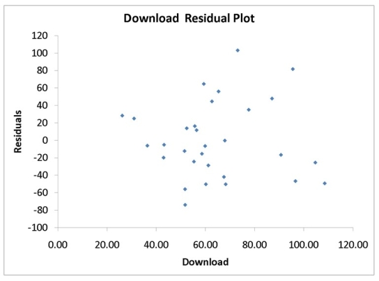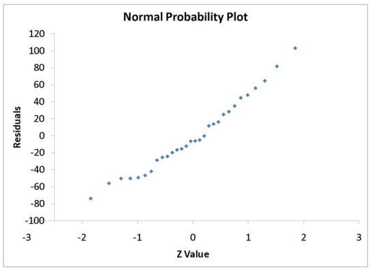-Referring to Instruction 12-11,which of the following assumptions appears to have been violated?

Instruction 12-4 The managers of a brokerage firm are interested in finding out if the number of new customers a broker brings into the firm affects the sales generated by the broker.They sample 12 brokers and determine the number of new customers they have enrolled in the last year and their sales amounts in thousands of dollars.These data are presented in the table that follows. Broker Clients Sales 1 27 52 2 11 37 3 42 64 4 33 55 5 15 29 6 15 34 7 25 58 8 36 59 9 28 44 10 30 48 11 17 31 12 22 38 -Referring to Instruction 12-4,the least squares estimate of the slope is ________.

Instruction 12-5 The managing partner of an advertising agency believes that his company's sales are related to the industry sales.He uses Microsoft Excel's Data Analysis tool to analyse the last four years of quarterly data with the following results: Regression Statistics Multiple R 0.802 R Square 0.643 Adjusted R Square 0.618 Standard Error SYX 0.9224 Observations 16 ANOVA df SS MS F Sig.F Regression 1 21.497 21.497 25.27 0.000 Error 14 11.912 0.851 Total 15 33.409 Predictor Coef StdError P-value Intercept 3.962 1.440 2.75 0.016 Industry 0.040451 0.008048 5.03 0.000 Durbin-Watson Statistic 1.59 -Referring to Instruction 12-5,the correlation coefficient is ________.

Instruction 12-4 The managers of a brokerage firm are interested in finding out if the number of new customers a broker brings into the firm affects the sales generated by the broker.They sample 12 brokers and determine the number of new customers they have enrolled in the last year and their sales amounts in thousands of dollars.These data are presented in the table that follows. Broker Clients Sales 1 27 52 2 11 37 3 42 64 4 33 55 5 15 29 6 15 34 7 25 58 8 36 59 9 28 44 10 30 48 11 17 31 12 22 38 -Referring to Instruction 12-4,the managers of the brokerage firm wanted to test the hypothesis that the number of new customers brought in did not affect the amount of sales generated.The value of the test statistic is ________.

Instruction 12-12 The manager of the purchasing department of a large savings and loan organization would like to develop a model to predict the amount of time (measured in hours)it takes to record a loan application.Data are collected from a sample of 30 days,and the number of applications recorded and completion time in hours is recorded.Below is the regression output: Regression Statistics Multiple R 0.9447 R Square 0.8924 Adjusted R 0.8886 Square Standard 0.3342 Error 30 Observations ANOVA df SS MS F Significance F Regression 1 25.9438 25.9438 232.2200 4.3946-15 Residual 28 3.1282 0.1117 Total 29 29.072 Coefficients Standard Error t Stat P -value Lower 95\% Upper 95\% Intercept Applications Recorded 0.4024 0.1236 3.2559 0.0030 0.1492 0.6555 Note: 4.3946E-15 is 4.3946 x 10^-15. -Referring to Instruction 12-12,the estimated mean amount of time it takes to record one additional loan application is

Instruction 12-4 The managers of a brokerage firm are interested in finding out if the number of new customers a broker brings into the firm affects the sales generated by the broker.They sample 12 brokers and determine the number of new customers they have enrolled in the last year and their sales amounts in thousands of dollars.These data are presented in the table that follows. Broker Clients Sales 1 27 52 2 11 37 3 42 64 4 33 55 5 15 29 6 15 34 7 25 58 8 36 59 9 28 44 10 30 48 11 17 31 12 22 38 -Referring to Instruction 12-4,suppose the managers of the brokerage firm want to obtain a 99% prediction interval for the sales made by a broker who has brought into the firm 18 new customers.The t critical value they would use is ________.

Instruction 12-10 The management of a chain electronic store would like to develop a model for predicting the weekly sales (in thousands of dollars)for individual stores based on the number of customers who made purchases.A random sample of 12 stores yields the following results: Customers Sales (Thousands of Dollars) 907 11.20 926 11.05 713 8.21 741 9.21 780 9.42 698 10.08 510 6.73 529 7.02 460 6.12 872 9.52 650 7.53 603 7.25 -Referring to Instruction 12-10,the value of the t test statistic and F test statistic should be the same when testing whether the number of customers who make purchases is a good predictor for weekly sales.

Instruction 12-5 The managing partner of an advertising agency believes that his company's sales are related to the industry sales.He uses Microsoft Excel's Data Analysis tool to analyse the last four years of quarterly data with the following results: Regression Statistics Multiple R 0.802 R Square 0.643 Adjusted R Square 0.618 Standard Error SYX 0.9224 Observations 16 ANOVA df SS MS F Sig.F Regression 1 21.497 21.497 25.27 0.000 Error 14 11.912 0.851 Total 15 33.409 Predictor Coef StdError t Stat P-value Intercept 3.962 1.440 2.75 0.016 Industry 0.040451 0.008048 5.03 0.000 Durbin-Watson Statistic 1.59 -Referring to Instruction 12-5,the partner wants to test for autocorrelation using the Durbin-Watson statistic.Using a level of significance of 0.05,the decision he should make is

Instruction 12-10 The management of a chain electronic store would like to develop a model for predicting the weekly sales (in thousands of dollars)for individual stores based on the number of customers who made purchases.A random sample of 12 stores yields the following results: Customers Sales (Thousands of Dollars) 907 11.20 926 11.05 713 8.21 741 9.21 780 9.42 698 10.08 510 6.73 529 7.02 460 6.12 872 9.52 650 7.53 603 7.25 -Referring to Instruction 12-10,what is the value of the coefficient of determination?

When using a regression model to make predictions,you should not predict Y for values of X larger or smaller than the values used to develop the model.

Instruction 12-9 It is believed that,the average numbers of hours spent studying per day (HOURS)during undergraduate education should have a positive linear relationship with the starting salary (SALARY,measured in thousands of dollars per month)after graduation.Given below is the Microsoft Excel output for predicting starting salary (Y)using number of hours spent studying per day (X)for a sample of 51 students.NOTE: Only partial output is shown. Regression Statistics Multiple R 0.8857 R Square 0.7845 Adjusted R Square 0.7801 Standard Error 1.3704 Observations 51 ANOVA df SS MS F Significance F Regression 1 335.0472 335.0473 178.3859 Residual 1.8782 Total 50 427.0798 Coefficients Standard Error t Stat P-value Lower 95\% Upper 95\% Intercept -1.8940 0.4018 -4.7134 2.051-05 -2.7015 -1.0865 Hours 0.9795 0.0733 13.3561 5.944-18 0.8321 1.1269 Note: 2.051E-05 = 2.051 * 10^-0.5 and 5.944E-18 = 5.944 * 10^-18. -Referring to Instruction 12-9,the degrees of freedom for the F test on whether HOURS affects SALARY are

Instruction 12-5 The managing partner of an advertising agency believes that his company's sales are related to the industry sales.He uses Microsoft Excel's Data Analysis tool to analyse the last four years of quarterly data with the following results: Regression Statistics Multiple R 0.802 R Square 0.643 Adjusted R Square 0.618 Standard Error SYX 0.9224 Observations 16 ANOVA df SS MS F Sig.F Regression 1 21.497 21.497 25.27 0.000 Error 14 11.912 0.851 Total 15 33.409 Predictor Coef StdError t Stat P-value Intercept 3.962 1.440 2.75 0.016 Industry 0.040451 0.008048 5.03 0.000 Durbin-Watson Statistic 1.59 -Referring to Instruction 12-5,the partner wants to test for autocorrelation using the Durbin-Watson statistic.Using a level of significance of 0.05,the critical values of the test are d_L = ________,and d_U = ________.

Instruction 12-1 A large national bank charges local companies for using their services.A bank official reported the results of a regression analysis designed to predict the bank's charges (Y)- measured in dollars per month - for services rendered to local companies.One independent variable used to predict service charge to a company is the company's sales revenue (X)- measured in millions of dollars.Data for 21 companies who use the bank's services were used to fit the model: Y₁ = β₀ + β₁X₁ + ε_i The results of the simple linear regression are provided below. $\hat { Y }$ = -2,700 + 20 X,S_YX = 65,two-tailed p value = 0.034 (for testing β₁) -Referring to Instruction 12-1,interpret the p-value for testing whether ?₁ exceeds 0.