Instruction 12-4 The managers of a brokerage firm are interested in finding out if the number of new customers a broker brings into the firm affects the sales generated by the broker.They sample 12 brokers and determine the number of new customers they have enrolled in the last year and their sales amounts in thousands of dollars.These data are presented in the table that follows. $\begin{array}{ccc} \text {Broker }&\text { Clients}&\text { Sales}\\ \hline1 & 27 & 52 \\ 2 & 11 & 37 \\ 3 & 42 & 64 \\ 4 & 33 & 55 \\ 5 & 15 & 29 \\ 6 & 15 & 34 \\ 7 & 25 & 58 \\ 8 & 36 & 59 \\ 9 & 28 & 44 \\ 10 & 30 & 48 \\ 11 & 17 & 31 \\ 12 & 22 & 38 \end{array}$ -Referring to Instruction 12-4,suppose the managers of the brokerage firm want to obtain a 99% confidence interval estimate for the mean sales made by brokers who have brought into the firm 24 new customers.The confidence interval is from ________ to ________.

The answer of Instruction 12-4 The managers of a brokerage firm...

Instruction 12-3 The director of cooperative education at a university wants to examine the effect of cooperative education job experience on marketability in the workplace.She takes a random sample of four students.For these four,she finds out how many times each had a cooperative education job and how many job offers they received upon graduation.These data are presented in the table below. \[\begin{array} { c c c } \text { Student } & \text { CoopJobs } & \text { JobOffer } \\ 1 & 1 & 4 \\ 2 & 2 & 6 \\ 3 & 1 & 3 \\ 4 & 0 & 1 \end{array}\] -Referring to Instruction 12-3,suppose the director of cooperative education wants to obtain a 95% confidence interval estimate for the mean number of job offers received by students who have had exactly one cooperative education job.The confidence interval is from ________ to ________.

The answer of Instruction 12-3 The director of cooperative education at...

Instruction 12-10 The management of a chain electronic store would like to develop a model for predicting the weekly sales (in thousands of dollars)for individual stores based on the number of customers who made purchases.A random sample of 12 stores yields the following results: \[\begin{array} { | c | c | } \hline \text { Customers } & \text { Sales (Thousands of Dollars) } \\ \hline 907 & 11.20 \\ \hline 926 & 11.05 \\ \hline 713 & 8.21 \\ \hline 741 & 9.21 \\ \hline 780 & 9.42 \\ \hline 698 & 10.08 \\ \hline 510 & 6.73 \\ \hline 529 & 7.02 \\ \hline 460 & 6.12 \\ \hline 872 & 9.52 \\ \hline 650 & 7.53 \\ \hline 603 & 7.25 \\ \hline \end{array}\] -Referring to Instruction 12-10,what is the value of the F test statistic when testing whether the number of customers who make purchases is a good predictor for weekly sales?

The answer of Instruction 12-10 The management of a chain electronic...

Instruction 12-10 The management of a chain electronic store would like to develop a model for predicting the weekly sales (in thousands of dollars)for individual stores based on the number of customers who made purchases.A random sample of 12 stores yields the following results: \[\begin{array} { | c | c | } \hline \text { Customers } & \text { Sales (Thousands of Dollars) } \\ \hline 907 & 11.20 \\ \hline 926 & 11.05 \\ \hline 713 & 8.21 \\ \hline 741 & 9.21 \\ \hline 780 & 9.42 \\ \hline 698 & 10.08 \\ \hline 510 & 6.73 \\ \hline 529 & 7.02 \\ \hline 460 & 6.12 \\ \hline 872 & 9.52 \\ \hline 650 & 7.53 \\ \hline 603 & 7.25 \\ \hline \end{array}\] -Referring to Instruction 12-10,generate the residual plot.

The answer of Instruction 12-10 The management of a chain electronic...

Exam 12: Simple Linear Regression

Instruction 12-3 The director of cooperative education at a university wants to examine the effect of cooperative education job experience on marketability in the workplace.She takes a random sample of four students.For these four,she finds out how many times each had a cooperative education job and how many job offers they received upon graduation.These data are presented in the table below. Student CoopJobs JobOffer 1 1 4 2 2 6 3 1 3 4 0 1 -Referring to Instruction 12-3,the coefficient of determination is ________.

(Short Answer)

4.8/5

(35)

Question 61

Instruction 12-4 The managers of a brokerage firm are interested in finding out if the number of new customers a broker brings into the firm affects the sales generated by the broker.They sample 12 brokers and determine the number of new customers they have enrolled in the last year and their sales amounts in thousands of dollars.These data are presented in the table that follows. Broker Clients Sales 1 27 52 2 11 37 3 42 64 4 33 55 5 15 29 6 15 34 7 25 58 8 36 59 9 28 44 10 30 48 11 17 31 12 22 38 -Referring to Instruction 12-4,suppose the managers of the brokerage firm want to obtain a 99% confidence interval estimate for the mean sales made by brokers who have brought into the firm 24 new customers.The confidence interval is from to .

(Short Answer)

4.7/5

(36)

Question 62

Instruction 12-2 A chocolate bar manufacturer is interested in trying to estimate how sales are influenced by the price of their product.To do this,the company randomly chooses six country towns and cities and offers the chocolate bar at different prices.Using chocolate bar sales as the dependent variable,the company will conduct a simple linear regression on the data below: City Price (\ ) Sales Toowoomba 1.30 100 Broken Hill 1.60 90 Bendigo 1.80 90 Kalgoorlie 2.00 40 Launceston 2.40 38 Port Augusta 2.90 32 -Referring to Instruction 12-2,if the price of the chocolate bar is set at $2,the estimated average sales will be

(Multiple Choice)

4.7/5

(29)

Question 63

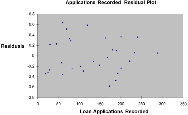
Instruction 12-12 The manager of the purchasing department of a large savings and loan organization would like to develop a model to predict the amount of time (measured in hours)it takes to record a loan application.Data are collected from a sample of 30 days,and the number of applications recorded and completion time in hours is recorded.Below is the regression output: Regression Statistics Multiple R 0.9447 R Square 0.8924 Adjusted R 0.8886 Square Standard 0.3342 Error 30 Observations ANOVA df SS MS F Significance F Regression 1 25.9438 25.9438 232.2200 4.3946-15 Residual 28 3.1282 0.1117 Total 29 29.072 Coefficients Standard Error t Stat P -value Lower 95\% Upper 95\% Intercept 0.4024 0.1236 3.2559 0.0030 0.1492 0.6555 Applications RECORD 0.0126 0.0008 15.2388 4.3946-15 0.0109 0.0143 Note: 4.3946E-15 is 4.3946 x 10^-15. $Instruction 12-12 The manager of the purchasing department of a large savings and loan organization would like to develop a model to predict the amount of time (measured in hours)it takes to record a loan application.Data are collected from a sample of 30 days,and the number of applications recorded and completion time in hours is recorded.Below is the regression output: \begin{array}{l} \begin{array} { l r } \hline { \text { Regression Statistics } } \\ \hline \text { Multiple R } & 0.9447 \\ \text { R Square } & 0.8924 \\ \text { Adjusted R } & 0.8886 \\ \text { Square } & \\ \text { Standard } & 0.3342 \\ \text { Error } & 30 \\ \text { Observations } & \\ \hline \end{array}\\ \text { ANOVA }\\ \begin{array} { l r r r r r } \hline & d f & { \text { SS } } & { \text { MS } } & F & { \begin{array} { c } \text { Significance } \\ F \end{array} } \\ \hline \text { Regression } & 1 & 25.9438 & 25.9438 & 232.2200 & 4.3946 \mathrm { E } - 15 \\ \text { Residual } & 28 & 3.1282 & 0.1117 & & \\ \text { Total } & 29 & 29.072 & & & \\ \hline \end{array}\\ \begin{array} { l r r r r r r } \hline & \text { Coefficients } & \begin{array} { c } \text { Standard } \\ \text { Error } \end{array} & t \text { Stat } & P \text {-value } & \text { Lower 95\% } & \text { Upper 95\% } \\ \text { Intercept } & 0.4024 & 0.1236 & 3.2559 & 0.0030 & 0.1492 & 0.6555 \\ \text { Applications RECORD } & 0.0126 & 0.0008 & 15.2388 & 4.3946 \mathrm{E}-15 & 0.0109 & 0.0143\\ \hline \end{array} \end{array} Note: 4.3946E-15 is 4.3946 x 10-15. -Referring to Instruction 12-12,you can be 95% confident that the mean amount of time needed to record one additional loan application is somewhere between 0.0109 and 0.0143 hours.$ $Instruction 12-12 The manager of the purchasing department of a large savings and loan organization would like to develop a model to predict the amount of time (measured in hours)it takes to record a loan application.Data are collected from a sample of 30 days,and the number of applications recorded and completion time in hours is recorded.Below is the regression output: \begin{array}{l} \begin{array} { l r } \hline { \text { Regression Statistics } } \\ \hline \text { Multiple R } & 0.9447 \\ \text { R Square } & 0.8924 \\ \text { Adjusted R } & 0.8886 \\ \text { Square } & \\ \text { Standard } & 0.3342 \\ \text { Error } & 30 \\ \text { Observations } & \\ \hline \end{array}\\ \text { ANOVA }\\ \begin{array} { l r r r r r } \hline & d f & { \text { SS } } & { \text { MS } } & F & { \begin{array} { c } \text { Significance } \\ F \end{array} } \\ \hline \text { Regression } & 1 & 25.9438 & 25.9438 & 232.2200 & 4.3946 \mathrm { E } - 15 \\ \text { Residual } & 28 & 3.1282 & 0.1117 & & \\ \text { Total } & 29 & 29.072 & & & \\ \hline \end{array}\\ \begin{array} { l r r r r r r } \hline & \text { Coefficients } & \begin{array} { c } \text { Standard } \\ \text { Error } \end{array} & t \text { Stat } & P \text {-value } & \text { Lower 95\% } & \text { Upper 95\% } \\ \text { Intercept } & 0.4024 & 0.1236 & 3.2559 & 0.0030 & 0.1492 & 0.6555 \\ \text { Applications RECORD } & 0.0126 & 0.0008 & 15.2388 & 4.3946 \mathrm{E}-15 & 0.0109 & 0.0143\\ \hline \end{array} \end{array} Note: 4.3946E-15 is 4.3946 x 10-15. -Referring to Instruction 12-12,you can be 95% confident that the mean amount of time needed to record one additional loan application is somewhere between 0.0109 and 0.0143 hours.$ -Referring to Instruction 12-12,you can be 95% confident that the mean amount of time needed to record one additional loan application is somewhere between 0.0109 and 0.0143 hours.

(True/False)

4.8/5

(32)

Question 64

Based on the residual plot below,you will conclude that there might be a violation of which of the following assumptions?

(Multiple Choice)

4.8/5

(23)

Question 65

Instruction 12-12 The manager of the purchasing department of a large savings and loan organization would like to develop a model to predict the amount of time (measured in hours)it takes to record a loan application.Data are collected from a sample of 30 days,and the number of applications recorded and completion time in hours is recorded.Below is the regression output: Regression Statistics Multiple R 0.9447 R Square 0.8924 Adjusted R 0.8886 Square Standard 0.3342 Error 30 Observations ANOVA df SS MS F Significance F Regression 1 25.9438 25.9438 232.2200 4.3946-15 Residual 28 3.1282 0.1117 Total 29 29.072 Coefficients Standard Error t Stat P -value Lower 95\% Upper 95\% Intercept 0.4024 0.1236 3.2559 0.0030 0.1492 0.6555 Applications RECORD 0.0126 0.0008 15.2388 4.3946-15 0.0109 0.0143 Note: 4.3946E-15 is 4.3946 x 10^-15. $Instruction 12-12 The manager of the purchasing department of a large savings and loan organization would like to develop a model to predict the amount of time (measured in hours)it takes to record a loan application.Data are collected from a sample of 30 days,and the number of applications recorded and completion time in hours is recorded.Below is the regression output: \begin{array}{l} \begin{array} { l r } \hline { \text { Regression Statistics } } \\ \hline \text { Multiple R } & 0.9447 \\ \text { R Square } & 0.8924 \\ \text { Adjusted R } & 0.8886 \\ \text { Square } & \\ \text { Standard } & 0.3342 \\ \text { Error } & 30 \\ \text { Observations } & \\ \hline \end{array}\\ \text { ANOVA }\\ \begin{array} { l r r r r r } \hline & d f & { \text { SS } } & { \text { MS } } & F & { \begin{array} { c } \text { Significance } \\ F \end{array} } \\ \hline \text { Regression } & 1 & 25.9438 & 25.9438 & 232.2200 & 4.3946 \mathrm { E } - 15 \\ \text { Residual } & 28 & 3.1282 & 0.1117 & & \\ \text { Total } & 29 & 29.072 & & & \\ \hline \end{array}\\ \begin{array} { l r r r r r r } \hline & \text { Coefficients } & \begin{array} { c } \text { Standard } \\ \text { Error } \end{array} & t \text { Stat } & P \text {-value } & \text { Lower 95\% } & \text { Upper 95\% } \\ \text { Intercept } & 0.4024 & 0.1236 & 3.2559 & 0.0030 & 0.1492 & 0.6555 \\ \text { Applications RECORD } & 0.0126 & 0.0008 & 15.2388 & 4.3946 \mathrm{E}-15 & 0.0109 & 0.0143\\ \hline \end{array} \end{array} Note: 4.3946E-15 is 4.3946 x 10-15. -Referring to Instruction 12-12,there is a 95% probability that the mean amount of time needed to record one additional loan application is somewhere between 0.0109 and 0.0143 hours.$ $Instruction 12-12 The manager of the purchasing department of a large savings and loan organization would like to develop a model to predict the amount of time (measured in hours)it takes to record a loan application.Data are collected from a sample of 30 days,and the number of applications recorded and completion time in hours is recorded.Below is the regression output: \begin{array}{l} \begin{array} { l r } \hline { \text { Regression Statistics } } \\ \hline \text { Multiple R } & 0.9447 \\ \text { R Square } & 0.8924 \\ \text { Adjusted R } & 0.8886 \\ \text { Square } & \\ \text { Standard } & 0.3342 \\ \text { Error } & 30 \\ \text { Observations } & \\ \hline \end{array}\\ \text { ANOVA }\\ \begin{array} { l r r r r r } \hline & d f & { \text { SS } } & { \text { MS } } & F & { \begin{array} { c } \text { Significance } \\ F \end{array} } \\ \hline \text { Regression } & 1 & 25.9438 & 25.9438 & 232.2200 & 4.3946 \mathrm { E } - 15 \\ \text { Residual } & 28 & 3.1282 & 0.1117 & & \\ \text { Total } & 29 & 29.072 & & & \\ \hline \end{array}\\ \begin{array} { l r r r r r r } \hline & \text { Coefficients } & \begin{array} { c } \text { Standard } \\ \text { Error } \end{array} & t \text { Stat } & P \text {-value } & \text { Lower 95\% } & \text { Upper 95\% } \\ \text { Intercept } & 0.4024 & 0.1236 & 3.2559 & 0.0030 & 0.1492 & 0.6555 \\ \text { Applications RECORD } & 0.0126 & 0.0008 & 15.2388 & 4.3946 \mathrm{E}-15 & 0.0109 & 0.0143\\ \hline \end{array} \end{array} Note: 4.3946E-15 is 4.3946 x 10-15. -Referring to Instruction 12-12,there is a 95% probability that the mean amount of time needed to record one additional loan application is somewhere between 0.0109 and 0.0143 hours.$ -Referring to Instruction 12-12,there is a 95% probability that the mean amount of time needed to record one additional loan application is somewhere between 0.0109 and 0.0143 hours.

(True/False)

4.8/5

(35)

Question 66

The residuals represent

(Multiple Choice)

4.8/5

(29)

Question 67

Instruction 12-3 The director of cooperative education at a university wants to examine the effect of cooperative education job experience on marketability in the workplace.She takes a random sample of four students.For these four,she finds out how many times each had a cooperative education job and how many job offers they received upon graduation.These data are presented in the table below. Student CoopJobs JobOffer 1 1 4 2 2 6 3 1 3 4 0 1 -Referring to Instruction 12-3,suppose the director of cooperative education wants to obtain a 95% confidence interval estimate for the mean number of job offers received by students who have had exactly one cooperative education job.The confidence interval is from to .

(Short Answer)

4.8/5

(32)

Question 68

Instruction 12-4 The managers of a brokerage firm are interested in finding out if the number of new customers a broker brings into the firm affects the sales generated by the broker.They sample 12 brokers and determine the number of new customers they have enrolled in the last year and their sales amounts in thousands of dollars.These data are presented in the table that follows. Broker Clients Sales 1 27 52 2 11 37 3 42 64 4 33 55 5 15 29 6 15 34 7 25 58 8 36 59 9 28 44 10 30 48 11 17 31 12 22 38 -Referring to Instruction 12-4,the standard error of the estimated slope coefficient is ________.

(Short Answer)

4.9/5

(34)

Question 69

Instruction 12-2 A chocolate bar manufacturer is interested in trying to estimate how sales are influenced by the price of their product.To do this,the company randomly chooses six country towns and cities and offers the chocolate bar at different prices.Using chocolate bar sales as the dependent variable,the company will conduct a simple linear regression on the data below: City Price (\ ) Sales Toowoomba 1.30 100 Broken Hill 1.60 90 Bendigo 1.80 90 Kalgoorlie 2.00 40 Launceston 2.40 38 Port Augusta 2.90 32 -Referring to Instruction 12-2,what is the coefficient of correlation for these data?

(Multiple Choice)

4.7/5

(31)

Question 70

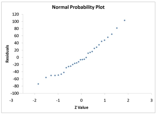
Instruction 12-11 A computer software developer would like to use the number of downloads (in thousands)for the trial version of his new shareware to predict the amount of revenue (in thousands of dollars)he can make on the full version of the new shareware.Following is the output from a simple linear regression along with the residual plot and normal probability plot obtained from a data set of 30 different sharewares that he has developed: Regression Statistics Multiple R 0.8691 R Square 0.7554 Adjusted R Square 0.7467 Standard Error 44.4765 Observations 30.0000 ANOVA df SS MS F significanceF Regression 1 171062.9193 171062.9193 86.4759 0.0000 Residual 28 55388.4309 1978.1582 Total 29 226451.3503 Coefficients Standard Error t Stat P-value Lower 95\% Upper 95\% Intercept -95.0614 26.9183 -3.5315 0.0015 -150.2009 -39.9218 Download 3.7297 0.4011 9.2992 0.0000 2.9082 4.5513 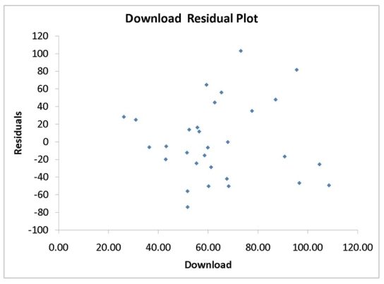$Instruction 12-11 A computer software developer would like to use the number of downloads (in thousands)for the trial version of his new shareware to predict the amount of revenue (in thousands of dollars)he can make on the full version of the new shareware.Following is the output from a simple linear regression along with the residual plot and normal probability plot obtained from a data set of 30 different sharewares that he has developed: \begin{array}{l|r} \hline {\text { Regression Statistics }} \\ \hline \text { Multiple R } & 0.8691 \\ \hline \text { R Square } & 0.7554 \\ \hline \text { Adjusted R Square } & 0.7467 \\ \hline \text { Standard Error } & 44.4765 \\ \hline \text { Observations } & 30.0000 \\ \hline \end{array} ANOVA \begin{array}{|l|r|r|r|r|r|} \hline &df&SS&MS&F&significance F\\ \hline \text { Regression } & 1 & 171062.9193 & 171062.9193 & 86.4759 & 0.0000 \\ \hline \text { Residual } & 28 & 55388.4309 & 1978.1582 & & \\ \hline \text { Total } & 29 & 226451.3503 & & & \\ \hline \end{array} \begin{array}{lrrrrrrr} \hline & \text { Coefficients } & \text { Standard Error } & t \text { Stat } & \text { P-value } & \text { Lower 95\% } & \text { Upper 95\% } \\ \hline \text { Intercept } & -95.0614 & 26.9183 & -3.5315 & 0.0015 & -150.2009 & -39.9218 \\ \text { Download } & 3.7297 & 0.4011 & 9.2992 & 0.0000 & 2.9082 & 4.5513 \\ \hline \end{array} -Referring to Instruction 12-11,which of the following is the correct interpretation for the slope coefficient?$ $Instruction 12-11 A computer software developer would like to use the number of downloads (in thousands)for the trial version of his new shareware to predict the amount of revenue (in thousands of dollars)he can make on the full version of the new shareware.Following is the output from a simple linear regression along with the residual plot and normal probability plot obtained from a data set of 30 different sharewares that he has developed: \begin{array}{l|r} \hline {\text { Regression Statistics }} \\ \hline \text { Multiple R } & 0.8691 \\ \hline \text { R Square } & 0.7554 \\ \hline \text { Adjusted R Square } & 0.7467 \\ \hline \text { Standard Error } & 44.4765 \\ \hline \text { Observations } & 30.0000 \\ \hline \end{array} ANOVA \begin{array}{|l|r|r|r|r|r|} \hline &df&SS&MS&F&significance F\\ \hline \text { Regression } & 1 & 171062.9193 & 171062.9193 & 86.4759 & 0.0000 \\ \hline \text { Residual } & 28 & 55388.4309 & 1978.1582 & & \\ \hline \text { Total } & 29 & 226451.3503 & & & \\ \hline \end{array} \begin{array}{lrrrrrrr} \hline & \text { Coefficients } & \text { Standard Error } & t \text { Stat } & \text { P-value } & \text { Lower 95\% } & \text { Upper 95\% } \\ \hline \text { Intercept } & -95.0614 & 26.9183 & -3.5315 & 0.0015 & -150.2009 & -39.9218 \\ \text { Download } & 3.7297 & 0.4011 & 9.2992 & 0.0000 & 2.9082 & 4.5513 \\ \hline \end{array} -Referring to Instruction 12-11,which of the following is the correct interpretation for the slope coefficient?$ -Referring to Instruction 12-11,which of the following is the correct interpretation for the slope coefficient?

(Multiple Choice)

4.9/5

(35)

Question 71

Instruction 12-11 A computer software developer would like to use the number of downloads (in thousands)for the trial version of his new shareware to predict the amount of revenue (in thousands of dollars)he can make on the full version of the new shareware.Following is the output from a simple linear regression along with the residual plot and normal probability plot obtained from a data set of 30 different sharewares that he has developed: Regression Statistics Multiple R 0.8691 R Square 0.7554 Adjusted R Square 0.7467 Standard Error 44.4765 Observations 30.0000 ANOVA df SS MS F significance F Regression 1 171062.9193 171062.9193 86.4759 0.0000 Residual 28 55388.4309 1978.1582 Total 29 226451.3503 Coefficients Standard Error t Stat P-value Lower 95\% Upper 95\% Intercept -95.0614 26.9183 -3.5315 0.0015 -150.2009 -39.9218 Download 3.7297 0.4011 9.2992 0.0000 2.9082 4.5513 $Instruction 12-11 A computer software developer would like to use the number of downloads (in thousands)for the trial version of his new shareware to predict the amount of revenue (in thousands of dollars)he can make on the full version of the new shareware.Following is the output from a simple linear regression along with the residual plot and normal probability plot obtained from a data set of 30 different sharewares that he has developed: \begin{array}{lr} \hline {\text { Regression Statistics }} \\ \hline \text { Multiple R } & 0.8691 \\ \hline \text { R Square } & 0.7554 \\ \hline \text { Adjusted R Square } & 0.7467 \\ \text { Standard Error } & 44.4765 \\ \text { Observations } & 30.0000 \end{array} ANOVA \begin{array}{|l|r|r|r|r|r|} \hline&df&SS&MS&F&\text {significance F}\\ \hline \text { Regression } & 1 & 171062.9193 & 171062.9193 & 86.4759 & 0.0000 \\ \hline \text { Residual } & 28 & 55388.4309 & 1978.1582 & & \\ \hline \text { Total } & 29 & 226451.3503 & &\\\hline \end{array} \begin{array}{lrrrrrrr} \hline & \text { Coefficients } & \text { Standard Error } & t \text { Stat } & \text { P-value } & \text { Lower 95\% } & \text { Upper 95\% } \\ \hline \text { Intercept } & -95.0614 & 26.9183 & -3.5315 & 0.0015 & -150.2009 & -39.9218 \\ \hline \text { Download } & 3.7297 & 0.4011 & 9.2992 & 0.0000 & 2.9082 & 4.5513 \end{array} -Referring to Instruction 12-11,the homoscedasticity of error assumption appears to have been violated.$ $Instruction 12-11 A computer software developer would like to use the number of downloads (in thousands)for the trial version of his new shareware to predict the amount of revenue (in thousands of dollars)he can make on the full version of the new shareware.Following is the output from a simple linear regression along with the residual plot and normal probability plot obtained from a data set of 30 different sharewares that he has developed: \begin{array}{lr} \hline {\text { Regression Statistics }} \\ \hline \text { Multiple R } & 0.8691 \\ \hline \text { R Square } & 0.7554 \\ \hline \text { Adjusted R Square } & 0.7467 \\ \text { Standard Error } & 44.4765 \\ \text { Observations } & 30.0000 \end{array} ANOVA \begin{array}{|l|r|r|r|r|r|} \hline&df&SS&MS&F&\text {significance F}\\ \hline \text { Regression } & 1 & 171062.9193 & 171062.9193 & 86.4759 & 0.0000 \\ \hline \text { Residual } & 28 & 55388.4309 & 1978.1582 & & \\ \hline \text { Total } & 29 & 226451.3503 & &\\\hline \end{array} \begin{array}{lrrrrrrr} \hline & \text { Coefficients } & \text { Standard Error } & t \text { Stat } & \text { P-value } & \text { Lower 95\% } & \text { Upper 95\% } \\ \hline \text { Intercept } & -95.0614 & 26.9183 & -3.5315 & 0.0015 & -150.2009 & -39.9218 \\ \hline \text { Download } & 3.7297 & 0.4011 & 9.2992 & 0.0000 & 2.9082 & 4.5513 \end{array} -Referring to Instruction 12-11,the homoscedasticity of error assumption appears to have been violated.$ -Referring to Instruction 12-11,the homoscedasticity of error assumption appears to have been violated.

(True/False)

5.0/5

(40)

Question 72

In performing a regression analysis involving two numerical variables,you are assuming

(Multiple Choice)

4.7/5

(34)

Question 73

Instruction 12-10 The management of a chain electronic store would like to develop a model for predicting the weekly sales (in thousands of dollars)for individual stores based on the number of customers who made purchases.A random sample of 12 stores yields the following results: Customers Sales (Thousands of Dollars) 907 11.20 926 11.05 713 8.21 741 9.21 780 9.42 698 10.08 510 6.73 529 7.02 460 6.12 872 9.52 650 7.53 603 7.25 -Referring to Instruction 12-10,what is the value of the F test statistic when testing whether the number of customers who make purchases is a good predictor for weekly sales?

(Short Answer)

4.8/5

(37)

Question 74

Instruction 12-10 The management of a chain electronic store would like to develop a model for predicting the weekly sales (in thousands of dollars)for individual stores based on the number of customers who made purchases.A random sample of 12 stores yields the following results: Customers Sales (Thousands of Dollars) 907 11.20 926 11.05 713 8.21 741 9.21 780 9.42 698 10.08 510 6.73 529 7.02 460 6.12 872 9.52 650 7.53 603 7.25 -Referring to Instruction 12-10,generate the residual plot.

(Essay)

4.9/5

(37)

Question 75

Instruction 12-3 The director of cooperative education at a university wants to examine the effect of cooperative education job experience on marketability in the workplace.She takes a random sample of four students.For these four,she finds out how many times each had a cooperative education job and how many job offers they received upon graduation.These data are presented in the table below. Student CoopJobs JobOffer 1 1 4 2 2 6 3 1 3 4 0 1 -Referring to Instruction 12-3,set up a scatter diagram.

(Essay)

4.8/5

(35)

Question 76

Instruction 12-2 A chocolate bar manufacturer is interested in trying to estimate how sales are influenced by the price of their product.To do this,the company randomly chooses six country towns and cities and offers the chocolate bar at different prices.Using chocolate bar sales as the dependent variable,the company will conduct a simple linear regression on the data below: City Price (\ ) Sales Toowoomba 1.30 100 Broken Hill 1.60 90 Bendigo 1.80 90 Kalgoorlie 2.00 40 Launceston 2.40 38 Port Augusta 2.90 32 -Referring to Instruction 12-2,what is the estimated average change in the sales of the chocolate bar if price goes up by $1.00?

(Multiple Choice)

4.9/5

(36)

Question 77

Instruction 12-12 The manager of the purchasing department of a large savings and loan organization would like to develop a model to predict the amount of time (measured in hours)it takes to record a loan application.Data are collected from a sample of 30 days,and the number of applications recorded and completion time in hours is recorded.Below is the regression output: Regression Statistics Multiple R 0.9447 R Square 0.8924 Adjusted R 0.8886 Square Standard 0.3342 Error 30 Observations ANOVA df SS MS F Significance F Regression 1 25.9438 25.9438 232.2200 4.3946-15 Residual 28 3.1282 0.1117 Total 29 29.072 Coefficients Standard Error t Stat P -value Lower 95\% Upper 95\% Intercept 0.4024 0.1236 3.2559 0.0030 0.1492 0.6555 Applications RECORD 0.0126 0.0008 15.2388 4.3946-15 0.0109 0.0143 Note: 4.3946E-15 is 4.3946 x 10^-15. $Instruction 12-12 The manager of the purchasing department of a large savings and loan organization would like to develop a model to predict the amount of time (measured in hours)it takes to record a loan application.Data are collected from a sample of 30 days,and the number of applications recorded and completion time in hours is recorded.Below is the regression output: \begin{array}{l} \begin{array} { l r } \hline { \text { Regression Statistics } } \\ \hline \text { Multiple R } & 0.9447 \\ \text { R Square } & 0.8924 \\ \text { Adjusted R } & 0.8886 \\ \text { Square } & \\ \text { Standard } & 0.3342 \\ \text { Error } & 30 \\ \text { Observations } & \\ \hline \end{array}\\ \text { ANOVA }\\ \begin{array} { l r r r r r } \hline & d f & { \text { SS } } & { \text { MS } } & F & { \begin{array} { c } \text { Significance } \\ F \end{array} } \\ \hline \text { Regression } & 1 & 25.9438 & 25.9438 & 232.2200 & 4.3946 \mathrm { E } - 15 \\ \text { Residual } & 28 & 3.1282 & 0.1117 & & \\ \text { Total } & 29 & 29.072 & & & \\ \hline \end{array}\\ \begin{array} { l r r r r r r } \hline & \text { Coefficients } & \begin{array} { c } \text { Standard } \\ \text { Error } \end{array} & t \text { Stat } & P \text {-value } & \text { Lower 95\% } & \text { Upper 95\% } \\ \text { Intercept } & 0.4024 & 0.1236 & 3.2559 & 0.0030 & 0.1492 & 0.6555 \\ \text { Applications RECORD } & 0.0126 & 0.0008 & 15.2388 & 4.3946 \mathrm{E}-15 & 0.0109 & 0.0143\\ \hline \end{array} \end{array} Note: 4.3946E-15 is 4.3946 x 10-15. -Referring to Instruction 12-12,the p-value of the measured t test statistic to test whether the number of loan applications recorded affects the amount of time is$ $Instruction 12-12 The manager of the purchasing department of a large savings and loan organization would like to develop a model to predict the amount of time (measured in hours)it takes to record a loan application.Data are collected from a sample of 30 days,and the number of applications recorded and completion time in hours is recorded.Below is the regression output: \begin{array}{l} \begin{array} { l r } \hline { \text { Regression Statistics } } \\ \hline \text { Multiple R } & 0.9447 \\ \text { R Square } & 0.8924 \\ \text { Adjusted R } & 0.8886 \\ \text { Square } & \\ \text { Standard } & 0.3342 \\ \text { Error } & 30 \\ \text { Observations } & \\ \hline \end{array}\\ \text { ANOVA }\\ \begin{array} { l r r r r r } \hline & d f & { \text { SS } } & { \text { MS } } & F & { \begin{array} { c } \text { Significance } \\ F \end{array} } \\ \hline \text { Regression } & 1 & 25.9438 & 25.9438 & 232.2200 & 4.3946 \mathrm { E } - 15 \\ \text { Residual } & 28 & 3.1282 & 0.1117 & & \\ \text { Total } & 29 & 29.072 & & & \\ \hline \end{array}\\ \begin{array} { l r r r r r r } \hline & \text { Coefficients } & \begin{array} { c } \text { Standard } \\ \text { Error } \end{array} & t \text { Stat } & P \text {-value } & \text { Lower 95\% } & \text { Upper 95\% } \\ \text { Intercept } & 0.4024 & 0.1236 & 3.2559 & 0.0030 & 0.1492 & 0.6555 \\ \text { Applications RECORD } & 0.0126 & 0.0008 & 15.2388 & 4.3946 \mathrm{E}-15 & 0.0109 & 0.0143\\ \hline \end{array} \end{array} Note: 4.3946E-15 is 4.3946 x 10-15. -Referring to Instruction 12-12,the p-value of the measured t test statistic to test whether the number of loan applications recorded affects the amount of time is$ -Referring to Instruction 12-12,the p-value of the measured t test statistic to test whether the number of loan applications recorded affects the amount of time is

(Multiple Choice)

4.8/5

(32)

Question 78

Instruction 12-10 The management of a chain electronic store would like to develop a model for predicting the weekly sales (in thousands of dollars)for individual stores based on the number of customers who made purchases.A random sample of 12 stores yields the following results: Customers Sales (Thousands of Dollars) 907 11.20 926 11.05 713 8.21 741 9.21 780 9.42 698 10.08 510 6.73 529 7.02 460 6.12 872 9.52 650 7.53 603 7.25 -Referring to Instruction 12-10,it is inappropriate to compute the Durbin-Watson statistic and test for autocorrelation in this case.

(True/False)

4.7/5

(34)

Question 79

Instruction 12-2 A chocolate bar manufacturer is interested in trying to estimate how sales are influenced by the price of their product.To do this,the company randomly chooses six country towns and cities and offers the chocolate bar at different prices.Using chocolate bar sales as the dependent variable,the company will conduct a simple linear regression on the data below: City Price (\ ) Sales Toowoomba 1.30 100 Broken Hill 1.60 90 Bendigo 1.80 90 Kalgoorlie 2.00 40 Launceston 2.40 38 Port Augusta 2.90 32 -Referring to Instruction 12-2,to test that the regression coefficient,?₁is not equal to 0,what would be the critical values? Use ? = 0.05.

(Multiple Choice)

4.9/5

(43)

Question 80

Showing 61 - 80 of 196

Based on the residual plot below,you will conclude that there might be a violation of which of the following assumptions?

The residuals represent

In performing a regression analysis involving two numerical variables,you are assuming

Introduction and Data Collection

Presenting Data in Tables and Charts

Numerical Descriptive Measures

Basic Probability

Some Important Discrete Probability Distributions

The Normal Distribution and Other Continuous Distributions

Sampling Distributions

Confidence Interval Estimation

Fundamentals of Hypothesis Testing: One-Sample Tests

Hypothesis Testing: Two Sample Tests

Analysis of Variance

Introduction to Multiple Regression

Time-Series Forecasting and Index Numbers

Chi-Square Tests

Multiple Regression Model Building

Decision Making

Statistical Applications in Quality and Productivity Management

Further Non-Parametric Tests

Filters