Exam 12: Simple Linear Regression

Instruction 12-12 The manager of the purchasing department of a large savings and loan organization would like to develop a model to predict the amount of time (measured in hours)it takes to record a loan application.Data are collected from a sample of 30 days,and the number of applications recorded and completion time in hours is recorded.Below is the regression output: Regression Statistics Multiple R 0.9447 R Square 0.8924 Adjusted R 0.8886 Square Standard 0.3342 Error 30 Observations ANOVA df SS MS F Significance F Regression 1 25.9438 25.9438 232.2200 4.3946-15 Residual 28 3.1282 0.1117 Total 29 29.072 Coefficients Standard Error t Stat P -value Lower 95\% Upper 95\% Intercept 0.4024 0.1236 3.2559 0.0030 0.1492 0.6555 Applications RECORD 0.0126 0.0008 15.2388 4.3946-15 0.0109 0.0143 Note: 4.3946E-15 is 4.3946 x 10^-15. 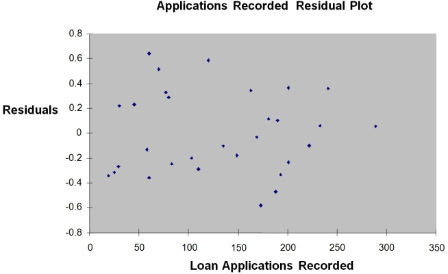-Referring to Instruction 12-12,there is sufficient evidence that the amount of time needed linearly depends on the number of loan applications at a 1% level of significance.

Instruction 12-4 The managers of a brokerage firm are interested in finding out if the number of new customers a broker brings into the firm affects the sales generated by the broker.They sample 12 brokers and determine the number of new customers they have enrolled in the last year and their sales amounts in thousands of dollars.These data are presented in the table that follows. Broker Clients Sales 1 27 52 2 11 37 3 42 64 4 33 55 5 15 29 6 15 34 7 25 58 8 36 59 9 28 44 10 30 48 11 17 31 12 22 38 -Referring to Instruction 12-4,the total sum of squares (SST)is ________.

Instruction 12-4 The managers of a brokerage firm are interested in finding out if the number of new customers a broker brings into the firm affects the sales generated by the broker.They sample 12 brokers and determine the number of new customers they have enrolled in the last year and their sales amounts in thousands of dollars.These data are presented in the table that follows. Broker Clients Sales 1 27 52 2 11 37 3 42 64 4 33 55 5 15 29 6 15 34 7 25 58 8 36 59 9 28 44 10 30 48 11 17 31 12 22 38 -Referring to Instruction 12-4,the coefficient of correlation is ________.

Instruction 12-4 The managers of a brokerage firm are interested in finding out if the number of new customers a broker brings into the firm affects the sales generated by the broker.They sample 12 brokers and determine the number of new customers they have enrolled in the last year and their sales amounts in thousands of dollars.These data are presented in the table that follows. Broker Clients Sales 1 27 52 2 11 37 3 42 64 4 33 55 5 15 29 6 15 34 7 25 58 8 36 59 9 28 44 10 30 48 11 17 31 12 22 38 -Referring to Instruction 12-4,the managers of the brokerage firm wanted to test the hypothesis that the true slope was equal to 0.At a level of significance of 0.01,the decision that should be made implies that ________ (there is or there is no)linear dependent relation between the independent and dependent variables.

The Y-intercept (b₀)represents the

Instruction 12-10 The management of a chain electronic store would like to develop a model for predicting the weekly sales (in thousands of dollars)for individual stores based on the number of customers who made purchases.A random sample of 12 stores yields the following results: Customers Sales (Thousands of Dollars) 907 11.20 926 11.05 713 8.21 741 9.21 780 9.42 698 10.08 510 6.73 529 7.02 460 6.12 872 9.52 650 7.53 603 7.25 -Referring to Instruction 12-10,the p-value of the t test and F test should be the same when testing whether the number of customers who make purchases is a good predictor for weekly sales.

When r = -1,it indicates a perfect relationship between X and Y.

Instruction 12-1 A large national bank charges local companies for using their services.A bank official reported the results of a regression analysis designed to predict the bank's charges (Y)- measured in dollars per month - for services rendered to local companies.One independent variable used to predict service charge to a company is the company's sales revenue (X)- measured in millions of dollars.Data for 21 companies who use the bank's services were used to fit the model: Y₁ = β₀ + β₁X₁ + ε_i The results of the simple linear regression are provided below. $\hat { Y }$ = -2,700 + 20 X,S_YX = 65,two-tailed p value = 0.034 (for testing β₁) -Referring to Instruction 12-1,interpret the estimate of ?,the standard deviation of the random error term (standard error of the estimate)in the model.

You give a pre-employment examination to your applicants.The test is scored from 1 to 100.You have data on their sales at the end of one year measured in dollars.You want to know if there is any linear relationship between pre-employment examination score and sales.An appropriate test to use is the t test on the population correlation coefficient.

The sample correlation coefficient between X and Y is 0.375.It has been found out that the p-value is 0.256 when testing H₀: ρ = 0 against the two-sided alternative H₁: ρ ≠ 0.To test H₀: ρ = 0 against the one-sided alternative H₁: ρ > 0 at a significance level of 0.2,the p-value is

The strength of the linear relationship between two numerical variables may be measured by the

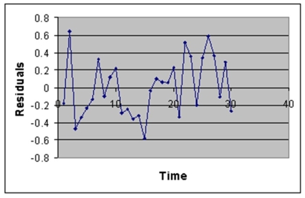
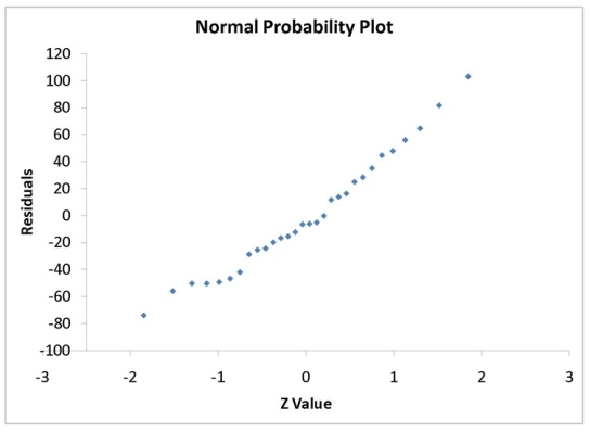
Instruction 12-11 A computer software developer would like to use the number of downloads (in thousands)for the trial version of his new shareware to predict the amount of revenue (in thousands of dollars)he can make on the full version of the new shareware.Following is the output from a simple linear regression along with the residual plot and normal probability plot obtained from a data set of 30 different sharewares that he has developed: Regression Statistics Multiple R 0.8691 R Square 0.7554 Adjusted R Square 0.7467 Standard Error 44.4765 Observations 30.0000 ANOVA df SS MS F Significance F Regression 1 171062.9193 171062.9193 86.4759 0.0000 Residual 28 55388.4309 1978.1582 Total 29 226451.3503 Coefficients Standard Error t Stat P-value Lower 95\% Upper 95\% Intercept -95.0614 26.9183 -3.5315 0.0015 -150.2009 -39.9218 Download 3.7297 0.4011 9.2992 0.0000 2.9082 4.5513 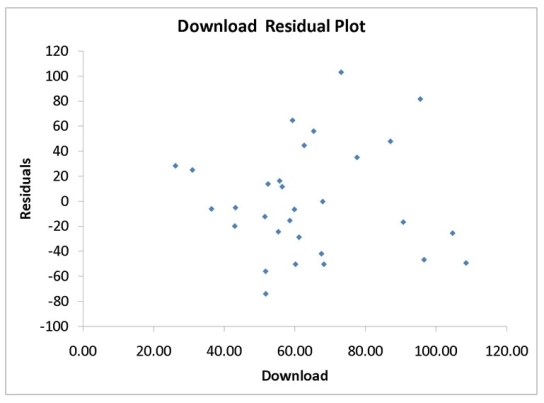-Referring to Instruction 12-11,there appears to be autocorrelation in the residuals.

Instruction 12-7 An investment specialist claims that if one holds a portfolio that moves in opposite direction to the market index like the All Ordinaries Index,then it is possible to reduce the variability of the portfolio's return.In other words,one can create a portfolio with positive returns but less exposure to risk.A sample of 26 years of the All Ordinaries index and a portfolio consisting of stocks of private prisons,which are believed to be negatively related to the All Ordinaries index,is collected.A regression analysis was performed by regressing the returns of the prison stocks portfolio (Y)on the returns of All Ordinaries index (X)to prove that the prison stocks portfolio is negatively related to the All Ordinaries index at a 5% level of significance.The results are given in the following Microsoft Excel output. Coefficients Standard Error T Stat P-value Intercept 4.866004258 0.35743609 13.61363441 8.7932-13 \& -0.502513506 0.071597152 -7.01862425 2.94942-07 -Referring to Instruction 12-7,to test whether the prison stocks portfolio is negatively related to the All Ordinaries index,the p-value of the associated test statistic is

Instruction 12-3 The director of cooperative education at a university wants to examine the effect of cooperative education job experience on marketability in the workplace.She takes a random sample of four students.For these four,she finds out how many times each had a cooperative education job and how many job offers they received upon graduation.These data are presented in the table below. Student CoopJobs JobOffer 1 1 4 2 2 6 3 1 3 4 0 1 -Referring to Instruction 12-3,the director of cooperative education wanted to test the hypothesis that the true slope was equal to 0.For a test with a level of significance of 0.05,the null hypothesis should be rejected if the value of the test statistic is ________.

The coefficient of determination (r²)tells you

Instruction 12-9 It is believed that,the average numbers of hours spent studying per day (HOURS)during undergraduate education should have a positive linear relationship with the starting salary (SALARY,measured in thousands of dollars per month)after graduation.Given below is the Microsoft Excel output for predicting starting salary (Y)using number of hours spent studying per day (X)for a sample of 51 students.NOTE: Only partial output is shown. Regression Statistics Multiple R 0.8857 R Square 0.7845 Adjusted R Square 0.7801 Standard Error 1.3704 Observations 51 ANOVA df SS MS F Significance F Regression 1 335.0472 335.0473 178.3859 Residual 1.8782 Total 50 427.0798 Coefficients Standard Error t Stat P-value Lower 95\% Upper 95\% Intercept -1.8940 0.4018 -4.7134 2.051-05 -2.7015 -1.0865 Hours 0.9795 0.0733 13.3561 5.944-18 0.8321 1.1269 Note: 2.051E-05 = 2.051 * 10^-0.5 and 5.944E-18 = 5.944 * 10^-18. -Referring to Instruction 12-9,the p-value of the measured F test statistic to test whether HOURS affects SALARY is

The Durbin-Watson D statistic is used to check the assumption of normality.

The Y-intercept (b₀)represents the

Instruction 12-9 It is believed that,the average numbers of hours spent studying per day (HOURS)during undergraduate education should have a positive linear relationship with the starting salary (SALARY,measured in thousands of dollars per month)after graduation.Given below is the Microsoft Excel output for predicting starting salary (Y)using number of hours spent studying per day (X)for a sample of 51 students.NOTE: Only partial output is shown. Regression Statistics Multiple R 0.8857 R Square 0.7845 Adjusted R Square 0.7801 Standard Error 1.3704 Observations 51 ANOVA df SS MS F Significance F Regression 1 335.0472 335.0473 178.3859 Residual 1.8782 Total 50 427.0798 Coefficients Standard Error t Stat P-value Lower 95\% Upper 95\% Intercept -1.8940 0.4018 -4.7134 2.051-05 -2.7015 -1.0865 Hours 0.9795 0.0733 13.3561 5.944-18 0.8321 1.1269 Note: 2.051E-05 = 2.051 * 10^-0.5 and 5.944E-18 = 5.944 * 10^-18. -Referring to Instruction 12-9,the 90% confidence interval for the average change in SALARY (in thousands of dollars)as a result of spending an extra hour per day studying is

Instruction 12-8 It is believed that average grade (based on a four -point scale)should have a positive linear relationship with university entrance exam scores.Given below is the Microsoft Excel output from regressing average grade on university entrance exam scores using a data set of eight randomly chosen students from a large university. Regressing average grade on university entrance exam score Regression Statistics Multiple R 0.7598 R Square 0.5774 Adjusted R Square 0.5069 Standard Error 0.2691 Observations 8 ANOVA df SS MS F Significance F Regression 1 0.5940 0.5940 8.1986 0.0286 Residual 6 0.4347 0.0724 Total 7 1.0287 Coefficients Standard Error t Stat P-value Lower 95\% Upper 95\% Intercept 0.5681 0.9284 0.6119 0.5630 -1.7036 2.8398 University entrance exam score 0.1021 0.0356 2.8633 0.0286 0.0148 0.1895 -Referring to Instruction 12-8,the value of the measured test statistic to test whether there is any linear relationship between average grade and university entrance exam score is