Exam 7: Scatterplots, Association, and Correlation
For the scenario described below, simply name the procedure that is appropriate to answer the question. For example,
1-proportion z-interval or chi-square goodness of fit test. Do NOT carry out the procedure.
-A flower pot manufacturer is testing his clay pots to ensure that the thickness of the sides are made to proper specifications. The sides are designed to be 4 mm thick. In a random sample of 25 pots, it is found that the average thickness if 4.3 mm. Does this provide statistically significant evidence that the manufacturing process is out of alignment?
1-mean t-test
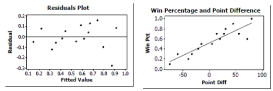
A sports analyst was interested in finding out how well a football team's winning percentage (stated as a proportion) can be predicted based upon points scored and points allowed. She selects a random sample of 15 football teams. Each team played 10 games. She decided to use the point differential, points scored minus points allowed as the predictor variable. The data are shown in the table below, and regression output is given afterward.
Point Diff Win Pct -75 .100 -60 .300 -40 .200 -33 .300 -21 .400 -15 .500 5 .500 14 .700 20 .600 28 .700 31 .800 45 .900 56 .700 72 .600 80 1.000
 Predictor Coef SE Coef T P Constant 0.51802 0.03071 16.87 0.000 Point Diff 0.0049500 0.0006682 7.41 0.000
Is there evidence of an association between Point Differential and Winning Percentage? Test an appropriate hypothesis and state your conclusion in the proper context.
Predictor Coef SE Coef T P Constant 0.51802 0.03071 16.87 0.000 Point Diff 0.0049500 0.0006682 7.41 0.000
Is there evidence of an association between Point Differential and Winning Percentage? Test an appropriate hypothesis and state your conclusion in the proper context.
We have Winning Percentage and Point Difference from a random sample of 15 teams. We want to know if there is an association between Winning Percentage and Point Difference.
H₀: There is no association between Winning Percentage and Point Difference. þ1 = 0
HA: There is an association between Winning Percentage and Point Difference. þ1 × 0
*Straight enough condition: There is no obvious bend in the original scatterplot of the data or in the plot of the residuals against the predicted values..
*Independence: These data were not collected over time and there is no pattern in the residuals plot.
*Does the plot thicken?: Neither the original scatterplot nor the residual plot shows any changes in the spread about the line.
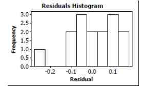
*Nearly Normal condition: With the exception of a possible outlier, the histogram of the residuals is roughly unimodal and symmetric.
Under these conditions the regression model is appropriate. We will use the linear regression t-test.
^
Regression equation: WinPct = 0.518 + 0.00495(PointDiff)
The for the regression is 80.8%. Point Difference seems to account for about 81% of the variability in Winning Percentage. The regression equation indicates that each additional 10 points in Point Difference corresponds to an increase in the Winning Percentage of about 0.05, on average.
The P-value < 0.0001 is very small, so we reject the null hypothesis. There is strong evidence of an association between Winning Percentage and Point Difference.
Production Workers at a large factory finish shirts with a hand sewn logo. The foreman overseeing the workers tracks the level of production. After collecting data for several months he estimates that workers complete an average of 230 shirts each day with a standard deviation of 13 shirts. He also believes that a normal model is appropriate to describe the distribution.
a) What is the probability that the workers will produce more than 250 shirts on a given
day?
b) Assuming that each day is independent, what are the chances that they will produce over 250 shirts for 3 days in a row?
a. z = 1.538; P(z > 1.538) = 0.062 b. (0.062)3 = 0.000238
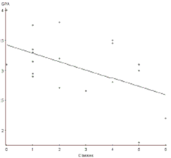
A San Jose State student collects data from 20 students. He compares the number of classes a student is enrolled in to their GPA. Here are the results of the regression analysis. The conditions for inference are satisfied.
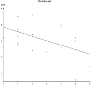 Simple linear regression results: Dependent Variable: GPA Sample size: 20
R-sq = 0.26753742 s: 0.45747
Coefficient Estimate Std. Err. T-Stat P-Value Constant 3.4246 0.16580 20.654 <0.0001 No. of Classes -0.13940 0.054369 -2.5641 0.0195
-What is the correlation coefficient for this relationship? Interpret this result in context.
Simple linear regression results: Dependent Variable: GPA Sample size: 20
R-sq = 0.26753742 s: 0.45747
Coefficient Estimate Std. Err. T-Stat P-Value Constant 3.4246 0.16580 20.654 <0.0001 No. of Classes -0.13940 0.054369 -2.5641 0.0195
-What is the correlation coefficient for this relationship? Interpret this result in context.
Cheater? A group of curious college students decide to test the integrity of their fellow collegians. In order to see if students will cheat, when given an opportunity, they decide to use chocolately M&M's. They tell each student that a discerning palette will be able to tell the difference in flavor between and red and a yellow candy. The blindfolded subjects are given two piles of candy to test. But the experimenter turns his back so that the subject thinks that they have a window of opportunity to take a quick peak. Unbeknownst to the subjects, there is another helper who is hidden and secretly watching to see who cheats. Here is their data. Cheated Did not cheat Male 6 2 Female 3 7
a. What is the probability that a subject cheated?
b. If a subject was a male, what are the chances that they cheated?
c. Using your answers to (a) and (b), does it appear that cheating and gender are
independent?
d. A statistics student in the group decides she wants to run a Chi-square test for independence. Why would this not be an advisable choice?
e. An argument begins. The girls are suggesting that the guys cheated more than girls; and
that this difference is larger than can be explained by chance variation. Of course, the guys insist that with a small sample size like this, anything could happen. Fortunately, a randomization machine is discovered. The 18 observations are randomly placed into the 4 categories randomly. This procedure is repeated 1000 times and the number of male
cheaters is counted each time. A graph is below. What does this graph tell you about the claims of the two groups? 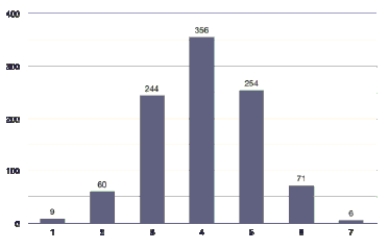
a. H0: There is no association between height and weight.
HA: There is an association between height and weight.
b. The scatterplot looks straight enough, residuals are random and display consistent spread, the histogram of
residuals looks roughly unimodal and symmetric.
c. Reject H? because of the small P-value; there is strong evidence of an association between height and weight. d. 7.30 ± 2.75
e. We are 95% confident that teenage boys gain an average of between 4.55 and 10.05 pounds per inch of height.
A college admissions counselor was interested in finding out how well high school grade point averages (HS GPA) predict first-year college GPAs (FY GPA). A random sample of data from first-year students was reviewed to obtain high school and first-year college GPAs. The data are shown below: HS GPA 3.82 3.90 3.20 3.40 3.88 3.50 3.60 3.70 FY GPA 3.75 3.45 2.60 2.95 3.50 2.76 3.10 3.40
HS GPA 4.00 3.30 3.50 3.80 3.87 4.00 3.20 3.82 FY GPA 3.90 2.70 3.00 3.00 3.10 3.77 2.80 3.54
Dependent variable is: FY GPA
No Selector
squared squared (adjusted)
with degrees of freedom
Source Sum of Squares df Mean Square F-ratio Regression 1.92283 1 1.92283 42.9 Residual 0.627867 14 0.044848 Variable Coefticient s.e. of Coeft t-ratio prob Constant -1.56410 0.7306 -2.14 0.0504 HS GPA 1.30527 0.1993 6.55 \leq0.0001
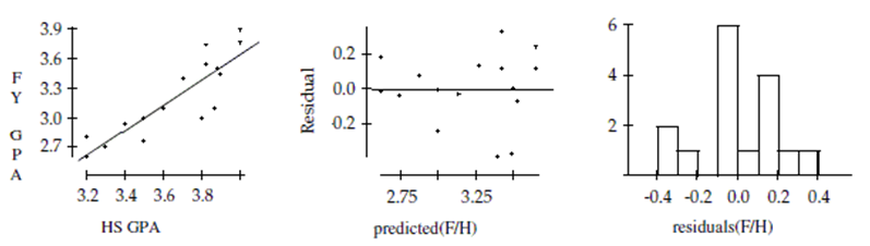 -Create and interpret a 95% confidence interval for the slope of the regression line.
For the scenario described below, simply name the procedure that is appropriate to answer the question. For example,
1-proportion z-interval or chi-square goodness of fit test. Do NOT carry out the procedure.
-A national marketing campaign is conducted to improve the name-brand recognition with potential customers. The company sells household products, primarily to the female head of the household. The current market analysis shows that 23% of their customer base recognizes the name of their product. When the marketing campaign is finished, 135
people out of 500 randomly polled recognize the brand name. Does this provide statistically significant evidence that there has been an increase in name-brand recognition?
A San Jose State student collects data from 20 students. He compares the number of classes a student is enrolled in to their GPA. Here are the results of the regression analysis. The conditions for inference are satisfied.
Simple linear regression results:
Dependent Variable: GPA
Sample size: 20
 Simple linear regression results: Dependent Variable: GPA Sample size: 20
R-sq = 0.26753742 s: 0.45747 Coefficient Estimate Std. Err. T-Stat P-Value Constant 3.4246 0.16580 20.654 <0.0001 No. of Classes -0.13940 0.054369 -2.5641 0.0195
-Is there evidence of a significant relationship between number of classes and GPA? Provide statistical justification for your answer.
Simple linear regression results: Dependent Variable: GPA Sample size: 20
R-sq = 0.26753742 s: 0.45747 Coefficient Estimate Std. Err. T-Stat P-Value Constant 3.4246 0.16580 20.654 <0.0001 No. of Classes -0.13940 0.054369 -2.5641 0.0195
-Is there evidence of a significant relationship between number of classes and GPA? Provide statistical justification for your answer.
A San Jose State student collects data from 20 students. He compares the number of classes a student is enrolled in to their GPA. Here are the results of the regression analysis. The conditions for inference are satisfied.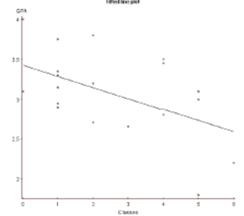 Simple linear regression results: Dependent Variable: GPA Sample size: 20
R-sq = 0.26753742 s: 0.45747
Coefficient Estimate Std. Err. T-Stat P-Value Constant 3.4246 0.16580 20.654 <0.0001 No. of Classes -0.13940 0.054369 -2.5641 0.0195
-Find and interpret a 95% confidence interval for the slope of the regression equation.
Simple linear regression results: Dependent Variable: GPA Sample size: 20
R-sq = 0.26753742 s: 0.45747
Coefficient Estimate Std. Err. T-Stat P-Value Constant 3.4246 0.16580 20.654 <0.0001 No. of Classes -0.13940 0.054369 -2.5641 0.0195
-Find and interpret a 95% confidence interval for the slope of the regression equation.
College admissions According to information from a college admissions office, 62% of the students there attended public high schools, 26% attended private high schools, 2% were home schooled, and the remaining students attended schools in other countries. Among this college's Honors Graduates last year there were 47 who came from public schools, 29 from private schools, 4 who had been home schooled, and 4 students from abroad. Is there any evidence that one type of high school might better equip students to attain high academic honors at this college? Test an appropriate hypothesis and state your conclusion.
Poverty In a study of how the burden of poverty varies among U.S. regions, a random sample of 1000 individuals from each region of the United States recently yielded the information on poverty (based on defining the poverty level as an income below $10,400 for a family of 4 people). The data are provided in the table below. (All the conditions are satisfied - don't worry about checking them.)
Northwest Midwest South West Total Poor 112 105 154 113 484 (121) (121) (121) (121) Not Poor 888 (879) 895 (879) 846 (879) 887 (879) 3516 Total 1000 1000 1000 1000 4000
=0.67+2.12+9.00+0.53+ 0.09+0.29+1.24+0.07+ =14.01
a. Write appropriate hypotheses.
b. How many degrees of freedom?
c. Suppose the expected values had not been given. Show exactly how to calculate the expected count in the first cell.
d. State your complete conclusion in context.
Car reliability A consumer group assigned 62 car models reliability ratings of 1 - 5 based upon repair records. They wondered if more expensive cars might be more reliable. To find out, they created the regression analysis shown. (SHOW WORK. Don't bother writing hypotheses, and you may assume the assumptions for inference were all satisfied.)
Dependent variable is: Reliability Variable Coefficient s.e. of coeff Constant 2.7029 0.3508 Price 0.5099 0.4116
a. df = ______, t = ______, P =______
b. State your conclusion.
How many degrees of freedom are there for regression inference with 28 data values?
Voter registration A random sample of 337 college students was asked whether or not they were registered to vote. We wonder if there is an association between a student's sex and whether the student is registered to vote. The data are provided in the table below
(expected counts are in parentheses). (All the conditions are satisfied - don't worry about checking them.) Men Women Total Registered 104(102) 147(149) 251 Not Registered 33(35) 53(51) 86 Total 137 200 337
a. Write appropriate hypotheses.
b. Suppose the expected values had not been given. Show exactly how to calculate the expected number of men who are registered to vote.
c. Show how to calculate the component of ç? for the first cell. d. How many degrees of freedom are there?
e. Find the P-value for this test.
f. State your complete conclusion in context.
As part of a survey, students in a large statistics class were asked whether or not they ate breakfast that morning. The data appears in the following table: Breakfast Yes No Total Sex Male 66 66 132 Female 125 74 199 Total 191 140 331
Is there evidence that eating breakfast is independent of the student's sex? Test an appropriate hypothesis. Give statistical evidence to support your conclusion.
In a local school, vending machines offer a range of drinks from juices to sports drinks. The purchasing agent thinks each type of drink is equally favored among the students buying drinks from the machines. The recent purchasing choices from the vending machines are shown in the table.
Drink Type/Flavor Lemon Lime Kiwi Tropical Grape Sports Drink Strawberry Punch Sports Drink Frequency 159 198 174 149
a. Test an appropriate hypothesis to decide if the purchasing agent is correct. Give statistical evidence to support your conclusion.
b. Which type of drink impacted your decision the most? Explain what this means in the
context of the problem.
A high school counselor was interested in finding out how well student grade point averages (GPA) predict ACT scores.
A sample of the senior class data was reviewed to obtain GPA and ACT scores. The data are shown in the table, and regression output is given below.
GPA ACT 3.25 24 2.87 21 2.66 18 3.33 22 2.87 22 3.21 22 2.76 18 3.91 28 3.55 29 2.55 18 2.44 20 3.22 24 3.01 21 3.44 24 3.22 25
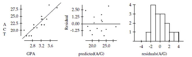 Dependent variable is:
No Selector
squared squared (adjusted)
with degrees of freedom
Source Sum of Squares df Mean Square F-ratio Regression 123.041 1 123.041 46.3 Residual 34.5589 13 2.65838 Variable Coefficient s.e. of Coeff t-ratio prob Constant -0.427035 3.382 -0.126 0.9014 GPA 7.39697 1.087 6.80 \leq0.0001
-Is there evidence of an association between GPA and ACT score? Test an appropriate hypothesis and state your conclusion in the proper context.
Dependent variable is:
No Selector
squared squared (adjusted)
with degrees of freedom
Source Sum of Squares df Mean Square F-ratio Regression 123.041 1 123.041 46.3 Residual 34.5589 13 2.65838 Variable Coefficient s.e. of Coeff t-ratio prob Constant -0.427035 3.382 -0.126 0.9014 GPA 7.39697 1.087 6.80 \leq0.0001
-Is there evidence of an association between GPA and ACT score? Test an appropriate hypothesis and state your conclusion in the proper context.
It's common for a movie's ticket sales to open high for the first couple of weeks, then gradually taper off as time passes. Hoping to be able to better understand how quickly sales decline, an industry analyst keeps track of box office revenues for a new film over its first 20 weeks. What inference method might provide useful insight?
A) -Interval for a mean
B) -test for linear regression
C) 1-proportion z-test
D) -Interval for slope
E) ç goodness-of-fit test
Wingspan A person's wingspan is the distance from fingertip to fingertip when their arms are fully extended. The longer a person's wingspan, the taller they tend to be. Regression analysis was executed on 24 individuals to see if height in inches can be used to predict wingspan (also in inches). The conditions for inference were deemed to be reasonably satisfied.
Dependent Variable: Wingspan
Sample size: 24
R-sq = 0.8026696 s: 2.1512606 Coefficient Estimate Std. Err. T-Stat P-Value Constant -13.024544 8.5719795 -1.5194324 0.1429 Height 1.1909246 0.125893 9.459816 <0.0001
a. Write the equation of the regression line. Make sure to define all the variables in your equation.
b. Interpret the slope of the regression equation in context. c. Interpret the value of s in context.
d. Find and interpret a 95% confidence interval for slope.
e. Is the relationship between wingspan and height a strong relationship? Why? Give two reasons to justify your answer.
^
Filters
- Essay(0)
- Multiple Choice(0)
- Short Answer(0)
- True False(0)
- Matching(0)