Exam 14: Introduction to Multiple Regression

arrow
  • Select Tags
search iconSearch Question
flashcardsStudy Flashcards
  • Select Tags

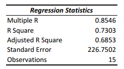
SCENARIO 14-10 You worked as an intern at We Always Win Car Insurance Company last summer. You notice that individual car insurance premiums depend very much on the age of the individual and the number of traffic tickets received by the individual. You performed a regression analysis in EXCEL and obtained the following partial information: SCENARIO 14-10 You worked as an intern at We Always Win Car Insurance Company last summer. You notice that individual car insurance premiums depend very much on the age of the individual and the number of traffic tickets received by the individual. You performed a regression analysis in EXCEL and obtained the following partial information:     -Referring to Scenario 14-10,to test the significance of the multiple regression model,the p- value of the test statistic in the sample is . SCENARIO 14-10 You worked as an intern at We Always Win Car Insurance Company last summer. You notice that individual car insurance premiums depend very much on the age of the individual and the number of traffic tickets received by the individual. You performed a regression analysis in EXCEL and obtained the following partial information:     -Referring to Scenario 14-10,to test the significance of the multiple regression model,the p- value of the test statistic in the sample is . -Referring to Scenario 14-10,to test the significance of the multiple regression model,the p- value of the test statistic in the sample is .
(Short Answer)
4.8/5
(43)

In a multiple regression model,the value of the coefficient of multiple determination

(Multiple Choice)
4.8/5
(33)

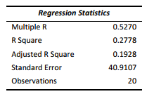
SCENARIO 14-6 One of the most common questions of prospective house buyers pertains to the cost of heating in dollars (Y). To provide its customers with information on that matter, a large real estate firm used the following 2 variables to predict heating costs: the daily minimum outside temperature in degrees of Fahrenheit ( X1 ) and the amount of insulation in inches ( X 2 ). Given below is EXCEL output of the regression model.  SCENARIO 14-6 One of the most common questions of prospective house buyers pertains to the cost of heating in dollars (Y). To provide its customers with information on that matter, a large real estate firm used the following 2 variables to predict heating costs: the daily minimum outside temperature in degrees of Fahrenheit ( X<sub>1</sub> ) and the amount of insulation in inches ( X <sub>2</sub> ). Given below is EXCEL output of the regression model.       Also SSR (X<sub>1</sub> | X<sub>2</sub>) = 8343.3572 and SSR (X<sub>2</sub> | X<sub>1</sub>) = 4199.2672 -Referring to Scenario 14-6,what is your decision and conclusion for the test H<sub>0 </sub>:  \beta <sub>2</sub> = 0 vs.H<sub>1 </sub>:  \beta <sub>2</sub>  \neq  0 at the  \alpha  = 0.01 level of significance?  SCENARIO 14-6 One of the most common questions of prospective house buyers pertains to the cost of heating in dollars (Y). To provide its customers with information on that matter, a large real estate firm used the following 2 variables to predict heating costs: the daily minimum outside temperature in degrees of Fahrenheit ( X<sub>1</sub> ) and the amount of insulation in inches ( X <sub>2</sub> ). Given below is EXCEL output of the regression model.       Also SSR (X<sub>1</sub> | X<sub>2</sub>) = 8343.3572 and SSR (X<sub>2</sub> | X<sub>1</sub>) = 4199.2672 -Referring to Scenario 14-6,what is your decision and conclusion for the test H<sub>0 </sub>:  \beta <sub>2</sub> = 0 vs.H<sub>1 </sub>:  \beta <sub>2</sub>  \neq  0 at the  \alpha  = 0.01 level of significance?  SCENARIO 14-6 One of the most common questions of prospective house buyers pertains to the cost of heating in dollars (Y). To provide its customers with information on that matter, a large real estate firm used the following 2 variables to predict heating costs: the daily minimum outside temperature in degrees of Fahrenheit ( X<sub>1</sub> ) and the amount of insulation in inches ( X <sub>2</sub> ). Given below is EXCEL output of the regression model.       Also SSR (X<sub>1</sub> | X<sub>2</sub>) = 8343.3572 and SSR (X<sub>2</sub> | X<sub>1</sub>) = 4199.2672 -Referring to Scenario 14-6,what is your decision and conclusion for the test H<sub>0 </sub>:  \beta <sub>2</sub> = 0 vs.H<sub>1 </sub>:  \beta <sub>2</sub>  \neq  0 at the  \alpha  = 0.01 level of significance? Also SSR (X1 | X2) = 8343.3572 and SSR (X2 | X1) = 4199.2672 -Referring to Scenario 14-6,what is your decision and conclusion for the test H0 : β\beta 2 = 0 vs.H1 : β\beta 2 \neq 0 at the α\alpha = 0.01 level of significance?
(Multiple Choice)
4.8/5
(36)

SCENARIO 14-8 A financial analyst wanted to examine the relationship between salary (in $1,000) and 2 variables: age (X1 = Age) and experience in the field (X2 = Exper). He took a sample of 20 employees and obtained the following Microsoft Excel output: SCENARIO 14-8 A financial analyst wanted to examine the relationship between salary (in $1,000) and 2 variables: age (X<sub>1</sub> = Age) and experience in the field (X<sub>2</sub> = Exper). He took a sample of 20 employees and obtained the following Microsoft Excel output:     Also, the sum of squares due to the regression for the model that includes only Age is 5022.0654 while the sum of squares due to the regression for the model that includes only Exper is 125.9848. -Referring to Scenario 14-8,the F test for the significance of the entire regression performed at a level of significance of 0.01 leads to a rejection of the null hypothesis. SCENARIO 14-8 A financial analyst wanted to examine the relationship between salary (in $1,000) and 2 variables: age (X<sub>1</sub> = Age) and experience in the field (X<sub>2</sub> = Exper). He took a sample of 20 employees and obtained the following Microsoft Excel output:     Also, the sum of squares due to the regression for the model that includes only Age is 5022.0654 while the sum of squares due to the regression for the model that includes only Exper is 125.9848. -Referring to Scenario 14-8,the F test for the significance of the entire regression performed at a level of significance of 0.01 leads to a rejection of the null hypothesis. Also, the sum of squares due to the regression for the model that includes only Age is 5022.0654 while the sum of squares due to the regression for the model that includes only Exper is 125.9848. -Referring to Scenario 14-8,the F test for the significance of the entire regression performed at a level of significance of 0.01 leads to a rejection of the null hypothesis.

(True/False)
4.9/5
(35)

SCENARIO 14-17 Given below are results from the regression analysis where the dependent variable is the number of weeks a worker is unemployed due to a layoff (Unemploy)and the independent variables are the age of the worker (Age)and a dummy variable for management position (Manager: 1 = yes,0 = no). The results of the regression analysis are given below: SCENARIO 14-17 Given below are results from the regression analysis where the dependent variable is the number of weeks a worker is unemployed due to a layoff (Unemploy)and the independent variables are the age of the worker (Age)and a dummy variable for management position (Manager: 1 = yes,0 = no). The results of the regression analysis are given below:     -Referring to Scenario 14-17,what are the numerator and denominator degrees of freedom,respectively,for the test statistic to determine whether there is a significant relationship between the number of weeks a worker is unemployed due to a layoff and the entire set of explanatory variables? SCENARIO 14-17 Given below are results from the regression analysis where the dependent variable is the number of weeks a worker is unemployed due to a layoff (Unemploy)and the independent variables are the age of the worker (Age)and a dummy variable for management position (Manager: 1 = yes,0 = no). The results of the regression analysis are given below:     -Referring to Scenario 14-17,what are the numerator and denominator degrees of freedom,respectively,for the test statistic to determine whether there is a significant relationship between the number of weeks a worker is unemployed due to a layoff and the entire set of explanatory variables? -Referring to Scenario 14-17,what are the numerator and denominator degrees of freedom,respectively,for the test statistic to determine whether there is a significant relationship between the number of weeks a worker is unemployed due to a layoff and the entire set of explanatory variables?

(Short Answer)
4.9/5
(34)

SCENARIO 14-17 Given below are results from the regression analysis where the dependent variable is the number of weeks a worker is unemployed due to a layoff (Unemploy)and the independent variables are the age of the worker (Age)and a dummy variable for management position (Manager: 1 = yes,0 = no). The results of the regression analysis are given below: SCENARIO 14-17 Given below are results from the regression analysis where the dependent variable is the number of weeks a worker is unemployed due to a layoff (Unemploy)and the independent variables are the age of the worker (Age)and a dummy variable for management position (Manager: 1 = yes,0 = no). The results of the regression analysis are given below:     -Referring to Scenario 14-17,which of the following is a correct statement? SCENARIO 14-17 Given below are results from the regression analysis where the dependent variable is the number of weeks a worker is unemployed due to a layoff (Unemploy)and the independent variables are the age of the worker (Age)and a dummy variable for management position (Manager: 1 = yes,0 = no). The results of the regression analysis are given below:     -Referring to Scenario 14-17,which of the following is a correct statement? -Referring to Scenario 14-17,which of the following is a correct statement?

(Multiple Choice)
4.7/5
(44)

SCENARIO 14-6 One of the most common questions of prospective house buyers pertains to the cost of heating in dollars (Y). To provide its customers with information on that matter, a large real estate firm used the following 2 variables to predict heating costs: the daily minimum outside temperature in degrees of Fahrenheit ( X1 ) and the amount of insulation in inches ( X 2 ). Given below is EXCEL output of the regression model. SCENARIO 14-6 One of the most common questions of prospective house buyers pertains to the cost of heating in dollars (Y). To provide its customers with information on that matter, a large real estate firm used the following 2 variables to predict heating costs: the daily minimum outside temperature in degrees of Fahrenheit ( X<sub>1</sub> ) and the amount of insulation in inches ( X <sub>2</sub> ). Given below is EXCEL output of the regression model.       Also SSR (X<sub>1</sub> | X<sub>2</sub>) = 8343.3572 and SSR (X<sub>2</sub> | X<sub>1</sub>) = 4199.2672 -Referring to Scenario 14-5,what is the p-value for testing whether Wages have a negative impact on corporate sales? SCENARIO 14-6 One of the most common questions of prospective house buyers pertains to the cost of heating in dollars (Y). To provide its customers with information on that matter, a large real estate firm used the following 2 variables to predict heating costs: the daily minimum outside temperature in degrees of Fahrenheit ( X<sub>1</sub> ) and the amount of insulation in inches ( X <sub>2</sub> ). Given below is EXCEL output of the regression model.       Also SSR (X<sub>1</sub> | X<sub>2</sub>) = 8343.3572 and SSR (X<sub>2</sub> | X<sub>1</sub>) = 4199.2672 -Referring to Scenario 14-5,what is the p-value for testing whether Wages have a negative impact on corporate sales? SCENARIO 14-6 One of the most common questions of prospective house buyers pertains to the cost of heating in dollars (Y). To provide its customers with information on that matter, a large real estate firm used the following 2 variables to predict heating costs: the daily minimum outside temperature in degrees of Fahrenheit ( X<sub>1</sub> ) and the amount of insulation in inches ( X <sub>2</sub> ). Given below is EXCEL output of the regression model.       Also SSR (X<sub>1</sub> | X<sub>2</sub>) = 8343.3572 and SSR (X<sub>2</sub> | X<sub>1</sub>) = 4199.2672 -Referring to Scenario 14-5,what is the p-value for testing whether Wages have a negative impact on corporate sales? Also SSR (X1 | X2) = 8343.3572 and SSR (X2 | X1) = 4199.2672 -Referring to Scenario 14-5,what is the p-value for testing whether Wages have a negative impact on corporate sales?

(Multiple Choice)
4.9/5
(28)

SCENARIO 14-13 An econometrician is interested in evaluating the relationship of demand for building materials to mortgage rates in Los Angeles and San Francisco.He believes that the appropriate model is Y = 10 + 5X1 + 8X2 where X1 = mortgage rate in % X2 = 1 if SF,0 if LA Y = demand in $100 per capita -Referring to Scenario 14-13,the fitted model for predicting demand in San Francisco is .

(Multiple Choice)
4.9/5
(33)

SCENARIO 14-17 Given below are results from the regression analysis where the dependent variable is the number of weeks a worker is unemployed due to a layoff (Unemploy)and the independent variables are the age of the worker (Age)and a dummy variable for management position (Manager: 1 = yes,0 = no). The results of the regression analysis are given below: SCENARIO 14-17 Given below are results from the regression analysis where the dependent variable is the number of weeks a worker is unemployed due to a layoff (Unemploy)and the independent variables are the age of the worker (Age)and a dummy variable for management position (Manager: 1 = yes,0 = no). The results of the regression analysis are given below:     -Referring to Scenario 14-17,what is the standard error of estimate? SCENARIO 14-17 Given below are results from the regression analysis where the dependent variable is the number of weeks a worker is unemployed due to a layoff (Unemploy)and the independent variables are the age of the worker (Age)and a dummy variable for management position (Manager: 1 = yes,0 = no). The results of the regression analysis are given below:     -Referring to Scenario 14-17,what is the standard error of estimate? -Referring to Scenario 14-17,what is the standard error of estimate?

(Short Answer)
5.0/5
(27)

SCENARIO 14-6 One of the most common questions of prospective house buyers pertains to the cost of heating in dollars (Y). To provide its customers with information on that matter, a large real estate firm used the following 2 variables to predict heating costs: the daily minimum outside temperature in degrees of Fahrenheit ( X1 ) and the amount of insulation in inches ( X 2 ). Given below is EXCEL output of the regression model. SCENARIO 14-6 One of the most common questions of prospective house buyers pertains to the cost of heating in dollars (Y). To provide its customers with information on that matter, a large real estate firm used the following 2 variables to predict heating costs: the daily minimum outside temperature in degrees of Fahrenheit ( X<sub>1</sub> ) and the amount of insulation in inches ( X <sub>2</sub> ). Given below is EXCEL output of the regression model.       Also SSR (X<sub>1</sub> | X<sub>2</sub>) = 8343.3572 and SSR (X<sub>2</sub> | X<sub>1</sub>) = 4199.2672 -Referring to Scenario 14-5,what is the p-value for testing whether Capital has a negative influence on corporate sales? SCENARIO 14-6 One of the most common questions of prospective house buyers pertains to the cost of heating in dollars (Y). To provide its customers with information on that matter, a large real estate firm used the following 2 variables to predict heating costs: the daily minimum outside temperature in degrees of Fahrenheit ( X<sub>1</sub> ) and the amount of insulation in inches ( X <sub>2</sub> ). Given below is EXCEL output of the regression model.       Also SSR (X<sub>1</sub> | X<sub>2</sub>) = 8343.3572 and SSR (X<sub>2</sub> | X<sub>1</sub>) = 4199.2672 -Referring to Scenario 14-5,what is the p-value for testing whether Capital has a negative influence on corporate sales? SCENARIO 14-6 One of the most common questions of prospective house buyers pertains to the cost of heating in dollars (Y). To provide its customers with information on that matter, a large real estate firm used the following 2 variables to predict heating costs: the daily minimum outside temperature in degrees of Fahrenheit ( X<sub>1</sub> ) and the amount of insulation in inches ( X <sub>2</sub> ). Given below is EXCEL output of the regression model.       Also SSR (X<sub>1</sub> | X<sub>2</sub>) = 8343.3572 and SSR (X<sub>2</sub> | X<sub>1</sub>) = 4199.2672 -Referring to Scenario 14-5,what is the p-value for testing whether Capital has a negative influence on corporate sales? Also SSR (X1 | X2) = 8343.3572 and SSR (X2 | X1) = 4199.2672 -Referring to Scenario 14-5,what is the p-value for testing whether Capital has a negative influence on corporate sales?

(Multiple Choice)
4.8/5
(26)

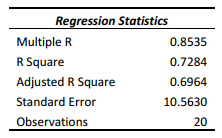
SCENARIO 14-8 A financial analyst wanted to examine the relationship between salary (in $1,000) and 2 variables: age (X1 = Age) and experience in the field (X2 = Exper). He took a sample of 20 employees and obtained the following Microsoft Excel output: SCENARIO 14-8 A financial analyst wanted to examine the relationship between salary (in $1,000) and 2 variables: age (X<sub>1</sub> = Age) and experience in the field (X<sub>2</sub> = Exper). He took a sample of 20 employees and obtained the following Microsoft Excel output:     Also, the sum of squares due to the regression for the model that includes only Age is 5022.0654 while the sum of squares due to the regression for the model that includes only Exper is 125.9848. -Referring to Scenario 14-8,the value of the partial F test statistic is _____ for H<sub>0</sub> : Variable X<sub>1</sub> does not significantly improve the model after variable X<sub>2</sub> has been included H<sub>1</sub> : Variable X<sub>1</sub> significantly improves the model after variable X<sub>2</sub> has been included SCENARIO 14-8 A financial analyst wanted to examine the relationship between salary (in $1,000) and 2 variables: age (X<sub>1</sub> = Age) and experience in the field (X<sub>2</sub> = Exper). He took a sample of 20 employees and obtained the following Microsoft Excel output:     Also, the sum of squares due to the regression for the model that includes only Age is 5022.0654 while the sum of squares due to the regression for the model that includes only Exper is 125.9848. -Referring to Scenario 14-8,the value of the partial F test statistic is _____ for H<sub>0</sub> : Variable X<sub>1</sub> does not significantly improve the model after variable X<sub>2</sub> has been included H<sub>1</sub> : Variable X<sub>1</sub> significantly improves the model after variable X<sub>2</sub> has been included Also, the sum of squares due to the regression for the model that includes only Age is 5022.0654 while the sum of squares due to the regression for the model that includes only Exper is 125.9848. -Referring to Scenario 14-8,the value of the partial F test statistic is _____ for H0 : Variable X1 does not significantly improve the model after variable X2 has been included H1 : Variable X1 significantly improves the model after variable X2 has been included
(Short Answer)
4.9/5
(40)

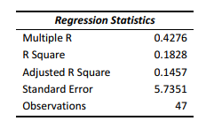
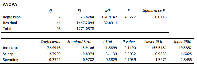
SCENARIO 14-15 The superintendent of a school district wanted to predict the percentage of students passing a sixthgrade proficiency test. She obtained the data on percentage of students passing the proficiency test (% Passing), mean teacher salary in thousands of dollars (Salaries), and instructional spending per pupil in thousands of dollars (Spending) of 47 schools in the state. Following is the multiple regression output with Y = % Passing as the dependent variable, X1 = Salaries and X 2 = Spending: SCENARIO 14-15 The superintendent of a school district wanted to predict the percentage of students passing a sixthgrade proficiency test. She obtained the data on percentage of students passing the proficiency test (% Passing), mean teacher salary in thousands of dollars (Salaries), and instructional spending per pupil in thousands of dollars (Spending) of 47 schools in the state. Following is the multiple regression output with Y = % Passing as the dependent variable, X<sub>1</sub> = Salaries and X <sub>2</sub> = Spending:     -Referring to Scenario 14-15,what are the lower and upper limits of the 95% confidence interval estimate for the effect of a one thousand dollars increase in instructional spending per pupil on the mean percentage of students passing the proficiency test? SCENARIO 14-15 The superintendent of a school district wanted to predict the percentage of students passing a sixthgrade proficiency test. She obtained the data on percentage of students passing the proficiency test (% Passing), mean teacher salary in thousands of dollars (Salaries), and instructional spending per pupil in thousands of dollars (Spending) of 47 schools in the state. Following is the multiple regression output with Y = % Passing as the dependent variable, X<sub>1</sub> = Salaries and X <sub>2</sub> = Spending:     -Referring to Scenario 14-15,what are the lower and upper limits of the 95% confidence interval estimate for the effect of a one thousand dollars increase in instructional spending per pupil on the mean percentage of students passing the proficiency test? -Referring to Scenario 14-15,what are the lower and upper limits of the 95% confidence interval estimate for the effect of a one thousand dollars increase in instructional spending per pupil on the mean percentage of students passing the proficiency test?

(Short Answer)
4.9/5
(37)

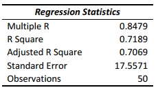
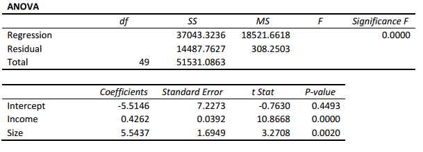
SCENARIO 14-4 A real estate builder wishes to determine how house size (House) is influenced by family income (Income) and family size (Size). House size is measured in hundreds of square feet and income is measured in thousands of dollars. The builder randomly selected 50 families and ran the multiple regression. Partial Microsoft Excel output is provided below: SCENARIO 14-4 A real estate builder wishes to determine how house size (House) is influenced by family income (Income) and family size (Size). House size is measured in hundreds of square feet and income is measured in thousands of dollars. The builder randomly selected 50 families and ran the multiple regression. Partial Microsoft Excel output is provided below:     Also SSR (X<sub>1</sub> | X<sub>2</sub>) = 36400.6326 and SSR (X<sub>1</sub> | X<sub>2</sub>) = 3297.7917 -Referring to Scenario 14-3,to test for the significance of the coefficient on gross domestic product,the p-value is SCENARIO 14-4 A real estate builder wishes to determine how house size (House) is influenced by family income (Income) and family size (Size). House size is measured in hundreds of square feet and income is measured in thousands of dollars. The builder randomly selected 50 families and ran the multiple regression. Partial Microsoft Excel output is provided below:     Also SSR (X<sub>1</sub> | X<sub>2</sub>) = 36400.6326 and SSR (X<sub>1</sub> | X<sub>2</sub>) = 3297.7917 -Referring to Scenario 14-3,to test for the significance of the coefficient on gross domestic product,the p-value is Also SSR (X1 | X2) = 36400.6326 and SSR (X1 | X2) = 3297.7917 -Referring to Scenario 14-3,to test for the significance of the coefficient on gross domestic product,the p-value is

(Multiple Choice)
4.8/5
(40)

In trying to construct a model to estimate grades on a statistics test,a professor wanted to include,among other factors,whether the person had taken the course previously.To do this,the professor included a dummy variable in her regression model that was equal to 1 if the person had previously taken the course,and 0 otherwise.The interpretation of the coefficient associated with this dummy variable would be the mean amount the repeat students tended to be above or below non-repeaters,with all other factors the same.

(True/False)
4.9/5
(35)

SCENARIO 14-15 The superintendent of a school district wanted to predict the percentage of students passing a sixthgrade proficiency test. She obtained the data on percentage of students passing the proficiency test (% Passing), mean teacher salary in thousands of dollars (Salaries), and instructional spending per pupil in thousands of dollars (Spending) of 47 schools in the state. Following is the multiple regression output with Y = % Passing as the dependent variable, X1 = Salaries and X 2 = Spending: SCENARIO 14-15 The superintendent of a school district wanted to predict the percentage of students passing a sixthgrade proficiency test. She obtained the data on percentage of students passing the proficiency test (% Passing), mean teacher salary in thousands of dollars (Salaries), and instructional spending per pupil in thousands of dollars (Spending) of 47 schools in the state. Following is the multiple regression output with Y = % Passing as the dependent variable, X<sub>1</sub> = Salaries and X <sub>2</sub> = Spending:     -Referring to Scenario 14-15,the null hypothesis should be rejected at a 5% level of significance when testing whether there is a significant relationship between percentage of students passing the proficiency test and the entire set of explanatory variables. SCENARIO 14-15 The superintendent of a school district wanted to predict the percentage of students passing a sixthgrade proficiency test. She obtained the data on percentage of students passing the proficiency test (% Passing), mean teacher salary in thousands of dollars (Salaries), and instructional spending per pupil in thousands of dollars (Spending) of 47 schools in the state. Following is the multiple regression output with Y = % Passing as the dependent variable, X<sub>1</sub> = Salaries and X <sub>2</sub> = Spending:     -Referring to Scenario 14-15,the null hypothesis should be rejected at a 5% level of significance when testing whether there is a significant relationship between percentage of students passing the proficiency test and the entire set of explanatory variables. -Referring to Scenario 14-15,the null hypothesis should be rejected at a 5% level of significance when testing whether there is a significant relationship between percentage of students passing the proficiency test and the entire set of explanatory variables.

(True/False)
4.7/5
(33)

SCENARIO 14-4 A real estate builder wishes to determine how house size (House) is influenced by family income (Income) and family size (Size). House size is measured in hundreds of square feet and income is measured in thousands of dollars. The builder randomly selected 50 families and ran the multiple regression. Partial Microsoft Excel output is provided below: SCENARIO 14-4 A real estate builder wishes to determine how house size (House) is influenced by family income (Income) and family size (Size). House size is measured in hundreds of square feet and income is measured in thousands of dollars. The builder randomly selected 50 families and ran the multiple regression. Partial Microsoft Excel output is provided below:     Also SSR (X<sub>1</sub> | X<sub>2</sub>) = 36400.6326 and SSR (X<sub>1</sub> | X<sub>2</sub>) = 3297.7917 -Referring to Scenario 14-4,the partial F test for H<sub>0</sub> : Variable X<sub>1</sub> does not significantly improve the model after variable X<sub>2</sub> has been included H<sub>1</sub> : Variable X<sub>1</sub> significantly improves the model after variable X<sub>2</sub> has been included has_____ and _____degrees of freedom. SCENARIO 14-4 A real estate builder wishes to determine how house size (House) is influenced by family income (Income) and family size (Size). House size is measured in hundreds of square feet and income is measured in thousands of dollars. The builder randomly selected 50 families and ran the multiple regression. Partial Microsoft Excel output is provided below:     Also SSR (X<sub>1</sub> | X<sub>2</sub>) = 36400.6326 and SSR (X<sub>1</sub> | X<sub>2</sub>) = 3297.7917 -Referring to Scenario 14-4,the partial F test for H<sub>0</sub> : Variable X<sub>1</sub> does not significantly improve the model after variable X<sub>2</sub> has been included H<sub>1</sub> : Variable X<sub>1</sub> significantly improves the model after variable X<sub>2</sub> has been included has_____ and _____degrees of freedom. Also SSR (X1 | X2) = 36400.6326 and SSR (X1 | X2) = 3297.7917 -Referring to Scenario 14-4,the partial F test for H0 : Variable X1 does not significantly improve the model after variable X2 has been included H1 : Variable X1 significantly improves the model after variable X2 has been included has_____ and _____degrees of freedom.

(Short Answer)
4.9/5
(31)

SCENARIO 14-8 A financial analyst wanted to examine the relationship between salary (in $1,000) and 2 variables: age (X1 = Age) and experience in the field (X2 = Exper). He took a sample of 20 employees and obtained the following Microsoft Excel output: SCENARIO 14-8 A financial analyst wanted to examine the relationship between salary (in $1,000) and 2 variables: age (X<sub>1</sub> = Age) and experience in the field (X<sub>2</sub> = Exper). He took a sample of 20 employees and obtained the following Microsoft Excel output:     Also, the sum of squares due to the regression for the model that includes only Age is 5022.0654 while the sum of squares due to the regression for the model that includes only Exper is 125.9848. -Referring to Scenario 14-8,the critical value of an F test on the entire regression for a level of significance of 0.01 is . SCENARIO 14-8 A financial analyst wanted to examine the relationship between salary (in $1,000) and 2 variables: age (X<sub>1</sub> = Age) and experience in the field (X<sub>2</sub> = Exper). He took a sample of 20 employees and obtained the following Microsoft Excel output:     Also, the sum of squares due to the regression for the model that includes only Age is 5022.0654 while the sum of squares due to the regression for the model that includes only Exper is 125.9848. -Referring to Scenario 14-8,the critical value of an F test on the entire regression for a level of significance of 0.01 is . Also, the sum of squares due to the regression for the model that includes only Age is 5022.0654 while the sum of squares due to the regression for the model that includes only Exper is 125.9848. -Referring to Scenario 14-8,the critical value of an F test on the entire regression for a level of significance of 0.01 is .

(Short Answer)
4.7/5
(39)

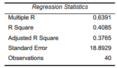
SCENARIO 14-17 Given below are results from the regression analysis where the dependent variable is the number of weeks a worker is unemployed due to a layoff (Unemploy)and the independent variables are the age of the worker (Age)and a dummy variable for management position (Manager: 1 = yes,0 = no). The results of the regression analysis are given below: SCENARIO 14-17 Given below are results from the regression analysis where the dependent variable is the number of weeks a worker is unemployed due to a layoff (Unemploy)and the independent variables are the age of the worker (Age)and a dummy variable for management position (Manager: 1 = yes,0 = no). The results of the regression analysis are given below:     -Referring to Scenario 14-17,we can conclude definitively that,holding constant the effect of the other independent variables,there is not a difference in the mean number of weeks a worker is unemployed due to a layoff between a worker who is in a management position and one who is not at a 10% level of significance if all we have is the information of the 95% confidence interval estimate for the difference in the mean number of weeks a worker is unemployed due to a layoff between a worker who is in a management position and one who is not. SCENARIO 14-17 Given below are results from the regression analysis where the dependent variable is the number of weeks a worker is unemployed due to a layoff (Unemploy)and the independent variables are the age of the worker (Age)and a dummy variable for management position (Manager: 1 = yes,0 = no). The results of the regression analysis are given below:     -Referring to Scenario 14-17,we can conclude definitively that,holding constant the effect of the other independent variables,there is not a difference in the mean number of weeks a worker is unemployed due to a layoff between a worker who is in a management position and one who is not at a 10% level of significance if all we have is the information of the 95% confidence interval estimate for the difference in the mean number of weeks a worker is unemployed due to a layoff between a worker who is in a management position and one who is not. -Referring to Scenario 14-17,we can conclude definitively that,holding constant the effect of the other independent variables,there is not a difference in the mean number of weeks a worker is unemployed due to a layoff between a worker who is in a management position and one who is not at a 10% level of significance if all we have is the information of the 95% confidence interval estimate for the difference in the mean number of weeks a worker is unemployed due to a layoff between a worker who is in a management position and one who is not.
(True/False)
4.9/5
(31)

The coefficient of multiple determination is calculated by taking the ratio of the regression sum of squares over the total sum of squares (SSR/SST)and subtracting that value from 1.

(True/False)
4.7/5
(28)

SCENARIO 14-8 A financial analyst wanted to examine the relationship between salary (in $1,000) and 2 variables: age (X1 = Age) and experience in the field (X2 = Exper). He took a sample of 20 employees and obtained the following Microsoft Excel output: SCENARIO 14-8 A financial analyst wanted to examine the relationship between salary (in $1,000) and 2 variables: age (X<sub>1</sub> = Age) and experience in the field (X<sub>2</sub> = Exper). He took a sample of 20 employees and obtained the following Microsoft Excel output:     Also, the sum of squares due to the regression for the model that includes only Age is 5022.0654 while the sum of squares due to the regression for the model that includes only Exper is 125.9848. -Referring to Scenario 14-7,the department head wants to use a t test to test for the significance of the coefficient of X<sub>1</sub>.For a level of significance of 0.05,the critical values of the test are . SCENARIO 14-8 A financial analyst wanted to examine the relationship between salary (in $1,000) and 2 variables: age (X<sub>1</sub> = Age) and experience in the field (X<sub>2</sub> = Exper). He took a sample of 20 employees and obtained the following Microsoft Excel output:     Also, the sum of squares due to the regression for the model that includes only Age is 5022.0654 while the sum of squares due to the regression for the model that includes only Exper is 125.9848. -Referring to Scenario 14-7,the department head wants to use a t test to test for the significance of the coefficient of X<sub>1</sub>.For a level of significance of 0.05,the critical values of the test are . Also, the sum of squares due to the regression for the model that includes only Age is 5022.0654 while the sum of squares due to the regression for the model that includes only Exper is 125.9848. -Referring to Scenario 14-7,the department head wants to use a t test to test for the significance of the coefficient of X1.For a level of significance of 0.05,the critical values of the test are .

(Short Answer)
4.8/5
(37)
Showing 181 - 200 of 256
close modal

Filters

  • Essay(0)
  • Multiple Choice(0)
  • Short Answer(0)
  • True False(0)
  • Matching(0)