Exam 14: Introduction to Multiple Regression

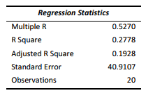
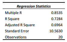
SCENARIO 14-8 A financial analyst wanted to examine the relationship between salary (in $1,000) and 2 variables: age (X₁ = Age) and experience in the field (X₂ = Exper). He took a sample of 20 employees and obtained the following Microsoft Excel output: 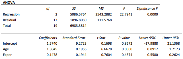Also, the sum of squares due to the regression for the model that includes only Age is 5022.0654 while the sum of squares due to the regression for the model that includes only Exper is 125.9848. -Referring to Scenario 14-8,the value of the adjusted coefficient of multiple determination is .

Using the hat matrix elements h_i to determine influential points in a multiple regression model with k independent variable and n observations,X_i is an influential point if

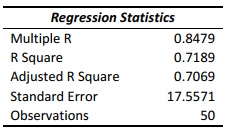
SCENARIO 14-4 A real estate builder wishes to determine how house size (House) is influenced by family income (Income) and family size (Size). House size is measured in hundreds of square feet and income is measured in thousands of dollars. The builder randomly selected 50 families and ran the multiple regression. Partial Microsoft Excel output is provided below: 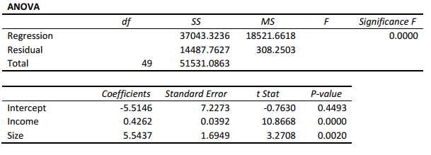Also SSR (X₁ | X₂) = 36400.6326 and SSR (X₁ | X₂) = 3297.7917 -Referring to Scenario 14-4,which of the following values for the level of significance is the smallest for which at least one explanatory variable is significant individually?

SCENARIO 14-15 The superintendent of a school district wanted to predict the percentage of students passing a sixthgrade proficiency test. She obtained the data on percentage of students passing the proficiency test (% Passing), mean teacher salary in thousands of dollars (Salaries), and instructional spending per pupil in thousands of dollars (Spending) of 47 schools in the state. 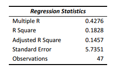Following is the multiple regression output with Y = % Passing as the dependent variable, X₁ = Salaries and X ₂ = Spending: 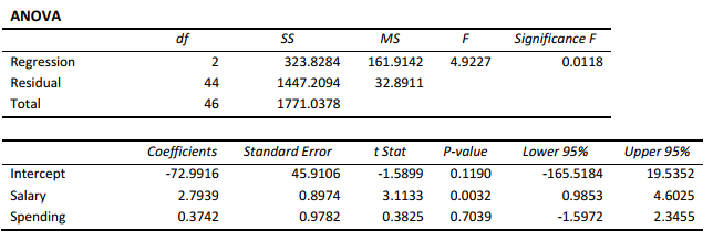-Referring to Scenario 14-15,there is sufficient evidence that the percentage of students passing the proficiency test depends on at least one of the explanatory variables at a 5% level of significance.

SCENARIO 14-13 An econometrician is interested in evaluating the relationship of demand for building materials to mortgage rates in Los Angeles and San Francisco.He believes that the appropriate model is Y = 10 + 5X₁ + 8X₂ where X₁ = mortgage rate in % X₂ = 1 if SF,0 if LA Y = demand in $100 per capita -Referring to Scenario 14-13,the effect of living in San Francisco rather than Los Angeles is to increase the mean demand by an estimated .

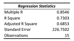
SCENARIO 14-6 One of the most common questions of prospective house buyers pertains to the cost of heating in dollars (Y). To provide its customers with information on that matter, a large real estate firm used the following 2 variables to predict heating costs: the daily minimum outside temperature in degrees of Fahrenheit ( X₁ ) and the amount of insulation in inches ( X ₂ ). Given below is EXCEL output of the regression model. 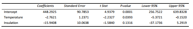Also SSR (X₁ | X₂) = 8343.3572 and SSR (X₂ | X₁) = 4199.2672 -Referring to Scenario 14-5,when the microeconomist used a simple linear regression model with sales as the dependent variable and wages as the independent variable,she obtained an r² value of 0.601.What additional percentage of the total variation of sales has been explained by including capital spending in the multiple regression?

A multiple regression is called "multiple" because it has several data points.

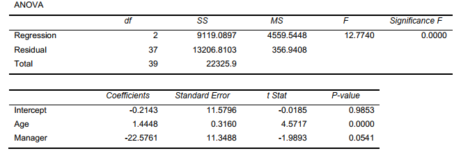
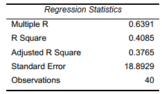
SCENARIO 14-17 Given below are results from the regression analysis where the dependent variable is the number of weeks a worker is unemployed due to a layoff (Unemploy)and the independent variables are the age of the worker (Age)and a dummy variable for management position (Manager: 1 = yes,0 = no). The results of the regression analysis are given below: -Referring to Scenario 14-17,estimate the mean number of weeks being unemployed due to a layoff for a worker who is a thirty-year old and is a manager.

SCENARIO 14-6 One of the most common questions of prospective house buyers pertains to the cost of heating in dollars (Y). To provide its customers with information on that matter, a large real estate firm used the following 2 variables to predict heating costs: the daily minimum outside temperature in degrees of Fahrenheit ( X₁ ) and the amount of insulation in inches ( X ₂ ). Given below is EXCEL output of the regression model. Also SSR (X₁ | X₂) = 8343.3572 and SSR (X₂ | X₁) = 4199.2672 -Referring to Scenario 14-5,the observed value of the F-statistic is given on the printout as 25.432.What are the degrees of freedom for this F-statistic?

SCENARIO 14-17 Given below are results from the regression analysis where the dependent variable is the number of weeks a worker is unemployed due to a layoff (Unemploy)and the independent variables are the age of the worker (Age)and a dummy variable for management position (Manager: 1 = yes,0 = no). The results of the regression analysis are given below: -Referring to Scenario 14-17,what is the p-value of the test statistic when testing whether age has any effect on the number of weeks a worker is unemployed due to a layoff while holding constant the effect of the other independent variable?

SCENARIO 14-10 You worked as an intern at We Always Win Car Insurance Company last summer. You notice that individual car insurance premiums depend very much on the age of the individual and the number of traffic tickets received by the individual. You performed a regression analysis in EXCEL and obtained the following partial information: 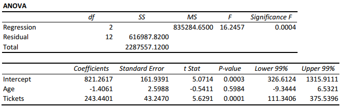-Referring to Scenario 14-10,the multiple regression model is significant at a 10% level of significance.

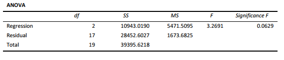
SCENARIO 14-8 A financial analyst wanted to examine the relationship between salary (in $1,000) and 2 variables: age (X₁ = Age) and experience in the field (X₂ = Exper). He took a sample of 20 employees and obtained the following Microsoft Excel output: Also, the sum of squares due to the regression for the model that includes only Age is 5022.0654 while the sum of squares due to the regression for the model that includes only Exper is 125.9848. -Referring to Scenario 14-8,the analyst wants to use a t test to test for the significance of the coefficient of X₂.The p-value of the test is .

SCENARIO 14-6 One of the most common questions of prospective house buyers pertains to the cost of heating in dollars (Y). To provide its customers with information on that matter, a large real estate firm used the following 2 variables to predict heating costs: the daily minimum outside temperature in degrees of Fahrenheit ( X₁ ) and the amount of insulation in inches ( X ₂ ). Given below is EXCEL output of the regression model. Also SSR (X₁ | X₂) = 8343.3572 and SSR (X₂ | X₁) = 4199.2672 -Referring to Scenario 14-6,the value of the partial F test statistic is _____ for H₀ : Variable X₁ does not significantly improve the model after variable X₂ has been included H₁ : Variable X₁ significantly improves the model after variable X₂ has been included

SCENARIO 14-17 Given below are results from the regression analysis where the dependent variable is the number of weeks a worker is unemployed due to a layoff (Unemploy)and the independent variables are the age of the worker (Age)and a dummy variable for management position (Manager: 1 = yes,0 = no). The results of the regression analysis are given below: -Referring to Scenario 14-17,what is the value of the test statistic to determine whether there is a significant relationship between the number of weeks a worker is unemployed due to a layoff and the entire set of explanatory variables?

Only when all three of the hat matrix elements h_i,the Studentized deleted residuals t_i and the Cook's distance statistic D_i reveal consistent result should an observation be removed from the regression analysis.

SCENARIO 14-15 The superintendent of a school district wanted to predict the percentage of students passing a sixthgrade proficiency test. She obtained the data on percentage of students passing the proficiency test (% Passing), mean teacher salary in thousands of dollars (Salaries), and instructional spending per pupil in thousands of dollars (Spending) of 47 schools in the state. Following is the multiple regression output with Y = % Passing as the dependent variable, X₁ = Salaries and X ₂ = Spending: -Referring to Scenario 14-15,which of the following is a correct statement?

SCENARIO 14-8 A financial analyst wanted to examine the relationship between salary (in $1,000) and 2 variables: age (X₁ = Age) and experience in the field (X₂ = Exper). He took a sample of 20 employees and obtained the following Microsoft Excel output: Also, the sum of squares due to the regression for the model that includes only Age is 5022.0654 while the sum of squares due to the regression for the model that includes only Exper is 125.9848. -Referring to Scenario 14-8,the analyst wants to use an F-test to test H₀ : $\beta$ ₁ = $\beta$ ₂ = 0 .The appropriate alternative hypothesis is .

SCENARIO 14-4 A real estate builder wishes to determine how house size (House) is influenced by family income (Income) and family size (Size). House size is measured in hundreds of square feet and income is measured in thousands of dollars. The builder randomly selected 50 families and ran the multiple regression. Partial Microsoft Excel output is provided below: Also SSR (X₁ | X₂) = 36400.6326 and SSR (X₁ | X₂) = 3297.7917 -Referring to Scenario 14-3,one economy in the sample had an aggregate consumption level of $4 billion,a GDP of $6 billion,and an aggregate price level of 200.What is the residual for this data point?

SCENARIO 14-8 A financial analyst wanted to examine the relationship between salary (in $1,000) and 2 variables: age (X₁ = Age) and experience in the field (X₂ = Exper). He took a sample of 20 employees and obtained the following Microsoft Excel output: Also, the sum of squares due to the regression for the model that includes only Age is 5022.0654 while the sum of squares due to the regression for the model that includes only Exper is 125.9848. -Referring to Scenario 14-8,the analyst wants to use a t test to test for the significance of the coefficient of X₂.For a level of significance of 0.01,the critical values of the test are .

SCENARIO 14-4 A real estate builder wishes to determine how house size (House) is influenced by family income (Income) and family size (Size). House size is measured in hundreds of square feet and income is measured in thousands of dollars. The builder randomly selected 50 families and ran the multiple regression. Partial Microsoft Excel output is provided below: Also SSR (X₁ | X₂) = 36400.6326 and SSR (X₁ | X₂) = 3297.7917 -Referring to Scenario 14-3,to test for the significance of the coefficient on aggregate price,the value of the relevant t-statistic is