Exam 16: Time-Series Forecasting

The fairly regular fluctuations that occur within each year would be contained in the _____ component.

SCENARIO 16-4 The number of cases of merlot wine sold by a Paso Robles winery in an 8-year period follows. 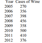-Referring to Scenario 16-3,if a three-month moving average is used to smooth this series,what would be the last calculated value?

Given a data set with 15 yearly observations,there are only seven 9-year moving averages.

SCENARIO 16-12 A local store developed a multiplicative time-series model to forecast its revenues in future quarters,using quarterly data on its revenues during the 5-year period from 2009 to 2013.The following is the resulting regression equation: log₁₀ Y^ˆ = 6.102 + 0.012 X - 0.129 Q₁ - 0.054 Q₂ + 0.098 Q₃ where Y^ˆ is the estimated number of contracts in a quarter. X is the coded quarterly value with X = 0 in the first quarter of 2008. Q₁ is a dummy variable equal to 1 in the first quarter of a year and 0 otherwise. Q₂ is a dummy variable equal to 1 in the second quarter of a year and 0 otherwise. Q₃ is a dummy variable equal to 1 in the third quarter of a year and 0 otherwise. Time-Series Forecasting 16-31 -Referring to Scenario 16-12,the best interpretation of the constant 6.102 in the regression equation is:

SCENARIO 16-4 The number of cases of merlot wine sold by a Paso Robles winery in an 8-year period follows. -Referring to Scenario 16-4,construct a centered 5-year moving average for the wine sales.

SCENARIO 16-12 A local store developed a multiplicative time-series model to forecast its revenues in future quarters,using quarterly data on its revenues during the 5-year period from 2009 to 2013.The following is the resulting regression equation: log₁₀ Y^ˆ = 6.102 + 0.012 X - 0.129 Q₁ - 0.054 Q₂ + 0.098 Q₃ where Y^ˆ is the estimated number of contracts in a quarter. X is the coded quarterly value with X = 0 in the first quarter of 2008. Q₁ is a dummy variable equal to 1 in the first quarter of a year and 0 otherwise. Q₂ is a dummy variable equal to 1 in the second quarter of a year and 0 otherwise. Q₃ is a dummy variable equal to 1 in the third quarter of a year and 0 otherwise. Time-Series Forecasting 16-31 -Referring to Scenario 16-12,the estimated quarterly compound growth rate in revenues is around:

The MAD is a measure of the mean of the absolute values of the deviations between the actual and the fitted values in a given time series.

SCENARIO 16-6 The president of a chain of department stores believes that her stores' total sales have been showing a linear trend since 1993.She uses Microsoft Excel to obtain the partial output below.The dependent variable is sales (in millions of dollars),while the independent variable is coded years,where 1993 is coded as 0,1994 is coded as 1,etc. 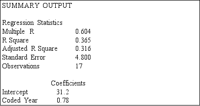-Referring to Scenario 16-6,the estimate of the amount by which sales (in millions of dollars)is increasing each year is .

SCENARIO 16-7 The executive vice-president of a drug manufacturing firm believes that the demand for the firm's most popular drug has been evidencing an exponential trend since 1999.She uses Microsoft Excel to obtain the partial output below.The dependent variable is the log base 10 of the demand for the drug,while the independent variable is years,where 1999 is coded as 0,2000 is coded as 1,etc. 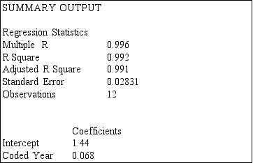-Referring to Scenario 16-7,the forecast for the demand in 2013 is .

SCENARIO 16-4 The number of cases of merlot wine sold by a Paso Robles winery in an 8-year period follows. -Referring to Scenario 16-4,exponential smoothing with a weight or smoothing constant of 0.2 will be used to forecast wine sales.The forecast for 2013 is .

SCENARIO 16-11 The manager of a health club has recorded mean attendance in newly introduced step classes over the last 15 months: 32.1,39.5,40.3,46.0,65.2,73.1,83.7,106.8,118.0,133.1,163.3,182.8, 205.6,249.1,and 263.5.She then used Microsoft Excel to obtain the following partial output for both a first- and second-order autoregressive model. -Referring to Scenario 16-11,using the first-order model,the forecast of mean attendance for month 16 is .

SCENARIO 16-14 A contractor developed a multiplicative time-series model to forecast the number of contracts in future quarters,using quarterly data on number of contracts during the 3-year period from 2011 to 2013.The following is the resulting regression equation: ln Y^ˆ = 3.37 + 0.117 X - 0.083 Q₁ + 1.28 Q₂ + 0.617 Q₃ where Y^ˆ is the estimated number of contracts in a quarter. X is the coded quarterly value with X = 0 in the first quarter of 2011. Q₁ is a dummy variable equal to 1 in the first quarter of a year and 0 otherwise. Q₂ is a dummy variable equal to 1 in the second quarter of a year and 0 otherwise. Q₃ is a dummy variable equal to 1 in the third quarter of a year and 0 otherwise. -Referring to Scenario 16-14,the best interpretation of the coefficient of X (0.117)in the regression equation is:

SCENARIO 16-7 The executive vice-president of a drug manufacturing firm believes that the demand for the firm's most popular drug has been evidencing an exponential trend since 1999.She uses Microsoft Excel to obtain the partial output below.The dependent variable is the log base 10 of the demand for the drug,while the independent variable is years,where 1999 is coded as 0,2000 is coded as 1,etc. -Referring to Scenario 16-7,the fitted exponential trend equation to predict Y is .

SCENARIO 16-4 The number of cases of merlot wine sold by a Paso Robles winery in an 8-year period follows. -Referring to Scenario 16-4,exponential smoothing with a weight or smoothing constant of 0.4 will be used to smooth the wine sales.The value of E₅,the smoothed value for 2009 is .

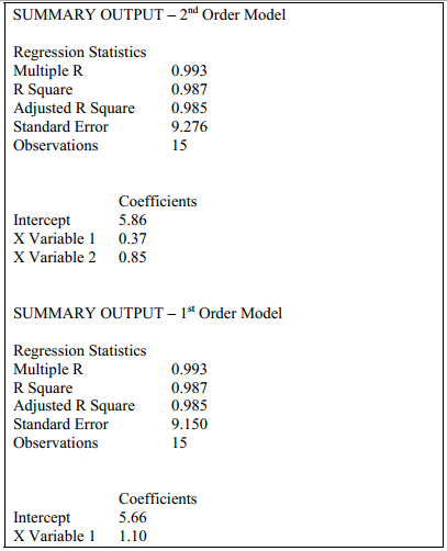
SCENARIO 16-10 Business closures in a city in the western U.S.from 2007 to 2012 were: Microsoft Excel was used to fit both first-order and second-order autoregressive models,resulting in the following partial outputs: -Referring to Scenario 16-10,the value of the MAD for the second-order autoregressive model is .

SCENARIO 16-10 Business closures in a city in the western U.S.from 2007 to 2012 were: Microsoft Excel was used to fit both first-order and second-order autoregressive models,resulting in the following partial outputs: -Referring to Scenario 16-10,the values of the MAD for the two models indicate that the first-order model should be used for forecasting.

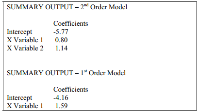
SCENARIO 16-13 Given below is the monthly time series data for U.S.retail sales of building materials over a specific year. The results of the linear trend,quadratic trend,exponential trend,first-order autoregressive,second-order autoregressive and third-order autoregressive model are presented below in which the coded month for the 1^st month is 0: Linear trend model: Quadratic trend model: Third-order autoregressive:: Below is the residual plot of the various models: 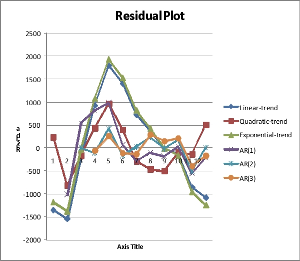-Referring to Scenario 16-13,the best model based on the residual plots is the exponential-trend regression model.

SCENARIO 16-13 Given below is the monthly time series data for U.S.retail sales of building materials over a specific year. The results of the linear trend,quadratic trend,exponential trend,first-order autoregressive,second-order autoregressive and third-order autoregressive model are presented below in which the coded month for the 1^st month is 0: Linear trend model: Quadratic trend model: Third-order autoregressive:: Below is the residual plot of the various models: -Referring to Scenario 16-13,what is the exponentially smoothed value for the second month using a smoothing coefficient of W = 0.25?

Given a data set with 15 yearly observations,a 3-year moving average will have fewer observations than a 5-year moving average.

The effect of an unpredictable,rare event will be contained in the _____ component.