Exam 18: A Roadmap for Analyzing Data

SCENARIO 18-12 The marketing manager for a nationally franchised lawn service company would like to study the characteristics that differentiate home owners who do and do not have a lawn service. A random sample of 30 home owners located in a suburban area near a large city was selected; 15 did not have a lawn service (code 0) and 15 had a lawn service (code 1). Additional information available concerning these 30 home owners includes family income (Income, in thousands of dollars), lawn size (Lawn Size, in thousands of square feet), attitude toward outdoor recreational activities (Attitude 0 = unfavorable, 1 = favorable), number of teenagers in the household (Teenager), and age of the head of the household (Age). The Minitab output is given below: 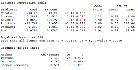-Referring to Scenario 18-12,the null hypothesis that the model is a good-fitting model cannot be rejected when allowing for a 5% probability of making a type I error.

SCENARIO 18-12 The marketing manager for a nationally franchised lawn service company would like to study the characteristics that differentiate home owners who do and do not have a lawn service. A random sample of 30 home owners located in a suburban area near a large city was selected; 15 did not have a lawn service (code 0) and 15 had a lawn service (code 1). Additional information available concerning these 30 home owners includes family income (Income, in thousands of dollars), lawn size (Lawn Size, in thousands of square feet), attitude toward outdoor recreational activities (Attitude 0 = unfavorable, 1 = favorable), number of teenagers in the household (Teenager), and age of the head of the household (Age). The Minitab output is given below: -Referring to Scenario 18-12,there is not enough evidence to conclude that Age makes a significant contribution to the model in the presence of the other independent variables at a 0.05 level of significance.

A certain type of rare gem serves as a status symbol for many of its owners.In theory,for low prices,the demand increases,and it decreases as the price of the gem increases.However,experts hypothesize that when the gem is valued at very high prices,the demand increases with price due to the status owners believe they gain in obtaining the gem.Data on price and quantity sold were collected for a sample of 35 rare gems of this type.Which of the following would be the most appropriate analysis to perform?

The quality control manager of a candy plant is inspecting a batch of chocolate chip bags.When the production process is in control,the average number of blue chocolate chips per bag is 6.0.Suppose that the probability of a blue chocolate chip in a bag is constant across bags and the number of blue chocolate chips in one bag is independent of the number in any other bag.Which of the following distributions would you use to figure out the probability that any particular bag being inspected has 4.0 blue chocolate chips?

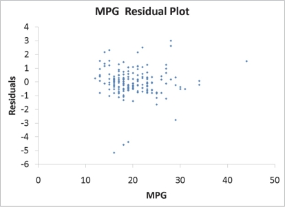
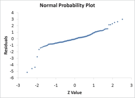
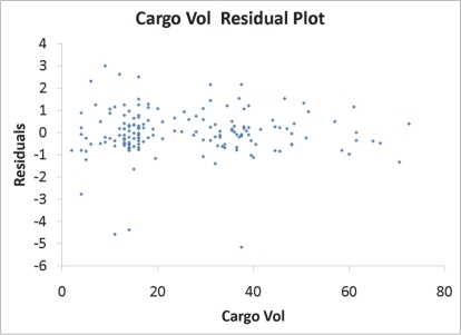
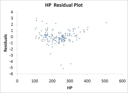
SCENARIO 18-9 What are the factors that determine the acceleration time (in sec. )from 0 to 60 miles per hour of a car? Data on the following variables for 171 different vehicle models were collected: Accel Time: Acceleration time in sec. Cargo Vol: Cargo volume in cu.ft. HP: Horsepower MPG: Miles per gallon SUV: 1 if the vehicle model is an SUV with Coupe as the base when SUV and Sedan are both 0 Sedan: 1 if the vehicle model is a sedan with Coupe as the base when SUV and Sedan are both 0 The regression results using acceleration time as the dependent variable and the remaining variables as the independent variables are presented below. The various residual plots are as shown below. 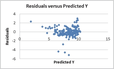The coefficient of partial determination ( R² _{yj.(All variables except j )} )of each of the 5 predictors are, respectively,0.0380,0.4376,0.0248,0.0188,and 0.0312. The coefficient of multiple determination for the regression model using each of the 5 variables X _j as the dependent variable and all other X variables as independent variables ( R² _j )are,respectively, 0.7461,0.5676,0.6764,0.8582,0.6632. -Referring to Scenario 18-9,_____of the variation in Accel Time can be explained by Cargo Vol while controlling for the other independent variables.

A powerful women's group has claimed that men and women differ in attitudes about sexual discrimination.A group of 50 men (group 1)and 40 women (group 2)were asked if they thought sexual discrimination is a problem in the United States.Of those sampled,11 of the men and 19 of the women did believe that sexual discrimination is a problem.Which of the following tests will you use to find out if there is any difference in attitudes about sexual discrimination?

Data on the amount of time spent studying and the exam score of 150 students at a high school were collected.You want to know if a student's exam score is linearly related to the amount of time spent on studying.Which of the following would you compute?

SCENARIO 18-2 One of the most common questions of prospective house buyers pertains to the cost of heating in dollars (Y). To provide its customers with information on that matter, a large real estate firm used the following 4 variables to predict heating costs: the daily minimum outside temperature in degrees of Fahrenheit ( X₁ ), the amount of insulation in inches ( X ₂ ), the number of windows in the house ( X₃ ), and the age of the furnace in years ( X ₄ ). Given below are the EXCEL outputs of two regression models. 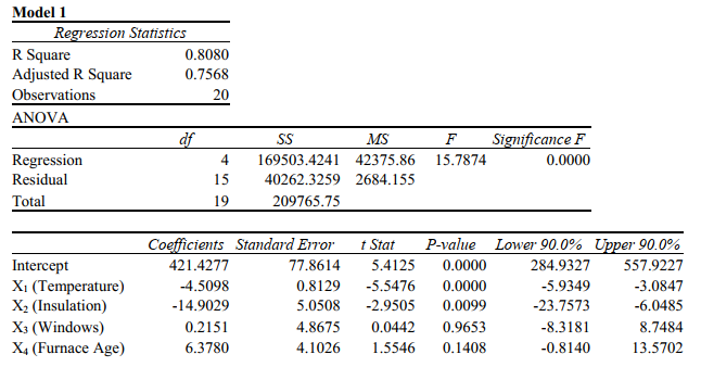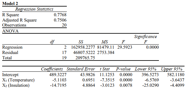-Referring to Scenario 18-2,what is the value of the partial F test statistic for H₀ : $\beta$ ₃ = $\beta$ ₄ = 0 vs. H₁ : At least one $\beta$ _j $\neq$ 0,j = 3,4 ?

SCENARIO 18-12 The marketing manager for a nationally franchised lawn service company would like to study the characteristics that differentiate home owners who do and do not have a lawn service. A random sample of 30 home owners located in a suburban area near a large city was selected; 15 did not have a lawn service (code 0) and 15 had a lawn service (code 1). Additional information available concerning these 30 home owners includes family income (Income, in thousands of dollars), lawn size (Lawn Size, in thousands of square feet), attitude toward outdoor recreational activities (Attitude 0 = unfavorable, 1 = favorable), number of teenagers in the household (Teenager), and age of the head of the household (Age). The Minitab output is given below: -Referring to Scenario 18-10 Model 1,the alternative hypothesis H₁ : At least one of $\beta$ _j $\neq$ 0 for j = 1,2,3,4,5,6 implies that the number of weeks a worker is unemployed due to a layoff is affected by at least one of the explanatory variables.

SCENARIO 18-9 What are the factors that determine the acceleration time (in sec. )from 0 to 60 miles per hour of a car? Data on the following variables for 171 different vehicle models were collected: Accel Time: Acceleration time in sec. Cargo Vol: Cargo volume in cu.ft. HP: Horsepower MPG: Miles per gallon SUV: 1 if the vehicle model is an SUV with Coupe as the base when SUV and Sedan are both 0 Sedan: 1 if the vehicle model is a sedan with Coupe as the base when SUV and Sedan are both 0 The regression results using acceleration time as the dependent variable and the remaining variables as the independent variables are presented below. The various residual plots are as shown below. The coefficient of partial determination ( R² _{yj.(All variables except j )} )of each of the 5 predictors are, respectively,0.0380,0.4376,0.0248,0.0188,and 0.0312. The coefficient of multiple determination for the regression model using each of the 5 variables X _j as the dependent variable and all other X variables as independent variables ( R² _j )are,respectively, 0.7461,0.5676,0.6764,0.8582,0.6632. -Referring to Scenario 18-9,the 0 to 60 miles per hour acceleration time of a coupe is predicted to be 0.7679 seconds lower than that of an SUV.

SCENARIO 18-2 One of the most common questions of prospective house buyers pertains to the cost of heating in dollars (Y). To provide its customers with information on that matter, a large real estate firm used the following 4 variables to predict heating costs: the daily minimum outside temperature in degrees of Fahrenheit ( X₁ ), the amount of insulation in inches ( X ₂ ), the number of windows in the house ( X₃ ), and the age of the furnace in years ( X ₄ ). Given below are the EXCEL outputs of two regression models. -Referring to Scenario 18-1,at the 0.01 level of significance,what conclusion should the builder reach regarding the inclusion of Income in the regression model?

SCENARIO 18-12 The marketing manager for a nationally franchised lawn service company would like to study the characteristics that differentiate home owners who do and do not have a lawn service. A random sample of 30 home owners located in a suburban area near a large city was selected; 15 did not have a lawn service (code 0) and 15 had a lawn service (code 1). Additional information available concerning these 30 home owners includes family income (Income, in thousands of dollars), lawn size (Lawn Size, in thousands of square feet), attitude toward outdoor recreational activities (Attitude 0 = unfavorable, 1 = favorable), number of teenagers in the household (Teenager), and age of the head of the household (Age). The Minitab output is given below: -Referring to Scenario 18-11,there is not enough evidence to conclude that SAT score makes a significant contribution to the model in the presence of the other independent variables at a 0.05 level of significance.

SCENARIO 18-6 A weight-loss clinic wants to use regression analysis to build a model for weight-loss of a client (measured in pounds).Two variables thought to affect weight-loss are client's length of time on the weight loss program and time of session.These variables are described below: 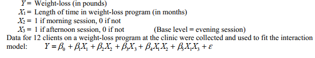Partial output from Microsoft Excel follows: 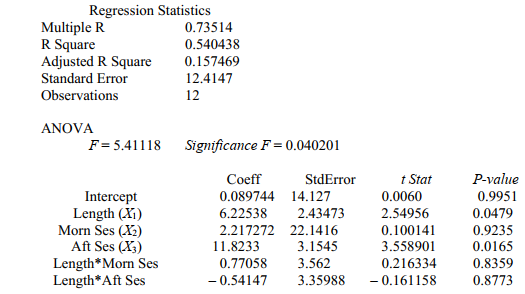-Referring to Scenario 18-6,in terms of the $\beta$ s in the model,give the mean change in weight- loss (Y)for every 1 month increase in time in the program (X₁)when attending the afternoon session.

SCENARIO 18-12 The marketing manager for a nationally franchised lawn service company would like to study the characteristics that differentiate home owners who do and do not have a lawn service. A random sample of 30 home owners located in a suburban area near a large city was selected; 15 did not have a lawn service (code 0) and 15 had a lawn service (code 1). Additional information available concerning these 30 home owners includes family income (Income, in thousands of dollars), lawn size (Lawn Size, in thousands of square feet), attitude toward outdoor recreational activities (Attitude 0 = unfavorable, 1 = favorable), number of teenagers in the household (Teenager), and age of the head of the household (Age). The Minitab output is given below: -Referring to Scenario 18-10 Model 1,which of the following is the correct alternative hypothesis to test whether being married or not makes a difference in the mean number of weeks a worker is unemployed due to a layoff while holding constant the effect of all the other independent variables?

A political pollster randomly selects a sample of 100 voters each day for 8 successive days and asks how many will vote for the incumbent.The pollster wishes to see if the percentage favoring the incumbent candidate is too erratic.Which of the following would be the most appropriate analysis to perform?

SCENARIO 18-9 What are the factors that determine the acceleration time (in sec. )from 0 to 60 miles per hour of a car? Data on the following variables for 171 different vehicle models were collected: Accel Time: Acceleration time in sec. Cargo Vol: Cargo volume in cu.ft. HP: Horsepower MPG: Miles per gallon SUV: 1 if the vehicle model is an SUV with Coupe as the base when SUV and Sedan are both 0 Sedan: 1 if the vehicle model is a sedan with Coupe as the base when SUV and Sedan are both 0 The regression results using acceleration time as the dependent variable and the remaining variables as the independent variables are presented below. The various residual plots are as shown below. The coefficient of partial determination ( R² _{yj.(All variables except j )} )of each of the 5 predictors are, respectively,0.0380,0.4376,0.0248,0.0188,and 0.0312. The coefficient of multiple determination for the regression model using each of the 5 variables X _j as the dependent variable and all other X variables as independent variables ( R² _j )are,respectively, 0.7461,0.5676,0.6764,0.8582,0.6632. -Referring to Scenario 18-9,_____of the variation in Accel Time can be explained by MPG while controlling for the other independent variables.

SCENARIO 18-12 The marketing manager for a nationally franchised lawn service company would like to study the characteristics that differentiate home owners who do and do not have a lawn service. A random sample of 30 home owners located in a suburban area near a large city was selected; 15 did not have a lawn service (code 0) and 15 had a lawn service (code 1). Additional information available concerning these 30 home owners includes family income (Income, in thousands of dollars), lawn size (Lawn Size, in thousands of square feet), attitude toward outdoor recreational activities (Attitude 0 = unfavorable, 1 = favorable), number of teenagers in the household (Teenager), and age of the head of the household (Age). The Minitab output is given below: -Referring to Scenario 18-11,what is the p-value of the test statistic when testing whether Toefl500 makes a significant contribution to the model in the presence of the other independent variables?

SCENARIO 18-8 The superintendent of a school district wanted to predict the percentage of students passing a sixth- grade proficiency test.She obtained the data on percentage of students passing the proficiency test (% Passing),daily mean of the percentage of students attending class (% Attendance),mean teacher salary in dollars (Salaries),and instructional spending per pupil in dollars (Spending)of 47 schools in the state. Following is the multiple regression output with Y = % Passing as the dependent variable, X₁ =% Attendance, X ₂ = Salaries and X₃ = Spending: 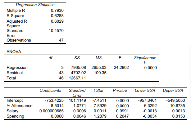-Referring to Scenario 18-8,there is sufficient evidence that daily mean of the percentage of students attending class has an effect on percentage of students passing the proficiency test while holding constant the effect of all the other independent variables at a 5% level of significance.

SCENARIO 18-12 The marketing manager for a nationally franchised lawn service company would like to study the characteristics that differentiate home owners who do and do not have a lawn service. A random sample of 30 home owners located in a suburban area near a large city was selected; 15 did not have a lawn service (code 0) and 15 had a lawn service (code 1). Additional information available concerning these 30 home owners includes family income (Income, in thousands of dollars), lawn size (Lawn Size, in thousands of square feet), attitude toward outdoor recreational activities (Attitude 0 = unfavorable, 1 = favorable), number of teenagers in the household (Teenager), and age of the head of the household (Age). The Minitab output is given below: -Referring to Scenario 18-10 Model 1,which of the following is the correct null hypothesis to test whether age has any effect on the number of weeks a worker is unemployed due to a layoff while holding constant the effect of all the other independent variables?

SCENARIO 18-12 The marketing manager for a nationally franchised lawn service company would like to study the characteristics that differentiate home owners who do and do not have a lawn service. A random sample of 30 home owners located in a suburban area near a large city was selected; 15 did not have a lawn service (code 0) and 15 had a lawn service (code 1). Additional information available concerning these 30 home owners includes family income (Income, in thousands of dollars), lawn size (Lawn Size, in thousands of square feet), attitude toward outdoor recreational activities (Attitude 0 = unfavorable, 1 = favorable), number of teenagers in the household (Teenager), and age of the head of the household (Age). The Minitab output is given below: -Referring to Scenario 18-10 Model 1,what is the value of the test statistic when testing whether age has any effect on the number of weeks a worker is unemployed due to a layoff while holding constant the effect of all the other independent variables?