Exam 12: Simple Linear Regression

If the plot of the residuals is fan shaped, which assumption is violated?

SCENARIO 12-12 The manager of the purchasing department of a large saving and loan organization would like to develop a model to predict the amount of time (measured in hours) it takes to record a loan application.Data are collected from a sample of 30 days, and the number of applications recorded and completion time in hours is recorded.Below is the regression output: Regression Statistics Multiple R 0.9447 R Square 0.8924 Adjusted R 0.8886 Square Standard 0.3342 Error Observations 30 ANOVA df SS MS F Significance F Regression 1 25.9438 25.9438 232.2200 4.3946-15 Residual 28 3.1282 0.1117 Total 29 29.072 Coefficients Standard Error t Stat P-value Lower 95\% Upper 95\% Intercept 0.4024 0.1236 3.2559 0.0030 0.1492 0.6555 Applications 0.0126 0.0008 15.2388 0.0000 0.0109 0.0143 Recorded 12-46 Simple Linear Regression 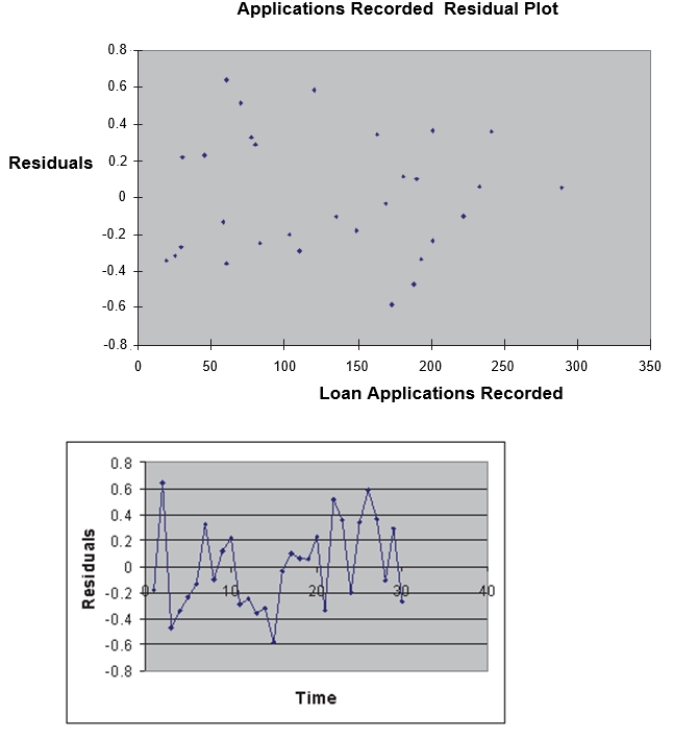Simple Linear Regression 12-47 -Referring to Scenario 12-12, the estimated mean amount of time it takes to record one additional loan application is

SCENARIO 12-3 The director of cooperative education at a state college wants to examine the effect of cooperative education job experience on marketability in the work place.She takes a random sample of 4 students.For these 4, she finds out how many times each had a cooperative education job and how many job offers they received upon graduation.These data are presented in the table below. Student Coop Jobs Job Offer 1 1 4 2 2 6 3 1 3 4 0 1 -Referring to Scenario 12-3, suppose the director of cooperative education wants to construct a95% prediction interval for the number of job offers received by a student who has had exactly two cooperative education jobs.The prediction interval is from to _.

SCENARIO 12-4 The managers of a brokerage firm are interested in finding out if the number of new clients a broker brings into the firm affects the sales generated by the broker.They sample 12 brokers and determine the number of new clients they have enrolled in the last year and their sales amounts in thousands of dollars.These data are presented in the table that follows. Broker Clients Sales 1 27 52 2 11 37 3 42 64 4 33 55 5 15 29 6 15 34 7 25 58 8 36 59 9 28 44 10 30 48 11 17 31 12 22 38 -Referring to Scenario 12-4, the prediction for the amount of sales (in $1,000s) for a person who brings 25 new clients into the firm is .

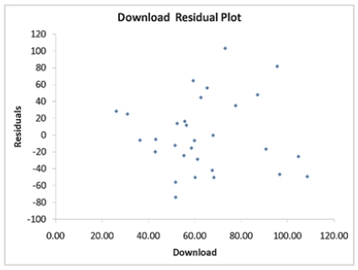
SCENARIO 12-11 A computer software developer would like to use the number of downloads (in thousands) for the trial version of his new shareware to predict the amount of revenue (in thousands of dollars) he can make on the full version of the new shareware.Following is the output from a simple linear regression along with the residual plot and normal probability plot obtained from a data set of 30 different sharewares that he has developed: Regression Statistics Multiple R 0.8691 R Square 0.7554 Adjusted R Square 0.7467 Standard Error 44.4765 Observations 30.0000 ANOVA df SS MS F Significance F Regression 1 171062.9193 171062.9193 86.4759 0.0000 Residual 28 55386.4309 1978.1582 Total 29 226451.3503 Coefficients Standard Error t Stat P-value Lower 95\% Upper 95\% Intercept -95.0614 26.9183 -3.5315 0.0015 -150.2009 -39.9218 Download 3.7297 0.4011 9.2992 0.0000 2.9082 4.5513 Simple Linear Regression 12-41 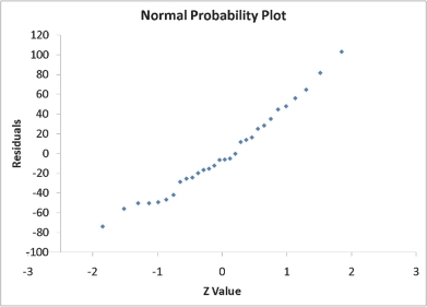-Referring to Scenario 12-11, what is the standard deviation around the regression line?

SCENARIO 12-4 The managers of a brokerage firm are interested in finding out if the number of new clients a broker brings into the firm affects the sales generated by the broker.They sample 12 brokers and determine the number of new clients they have enrolled in the last year and their sales amounts in thousands of dollars.These data are presented in the table that follows. Broker Clients Sales 1 27 52 2 11 37 3 42 64 4 33 55 5 15 29 6 15 34 7 25 58 8 36 59 9 28 44 10 30 48 11 17 31 12 22 38 -Referring to Scenario 12-4, the standard error of the estimated slope coefficient is _.

SCENARIO 12-4 The managers of a brokerage firm are interested in finding out if the number of new clients a broker brings into the firm affects the sales generated by the broker.They sample 12 brokers and determine the number of new clients they have enrolled in the last year and their sales amounts in thousands of dollars.These data are presented in the table that follows. Broker Clients Sales 1 27 52 2 11 37 3 42 64 4 33 55 5 15 29 6 15 34 7 25 58 8 36 59 9 28 44 10 30 48 11 17 31 12 22 38 -Referring to Scenario 12-4, % of the total variation in sales generated can be explained by the number of new clients brought in.

SCENARIO 12-12 The manager of the purchasing department of a large saving and loan organization would like to develop a model to predict the amount of time (measured in hours) it takes to record a loan application.Data are collected from a sample of 30 days, and the number of applications recorded and completion time in hours is recorded.Below is the regression output: Regression Statistics Multiple R 0.9447 R Square 0.8924 Adjusted R 0.8886 Square Standard 0.3342 Error Observations 30 ANOVA df SS MS F Significance F Regression 1 25.9438 25.9438 232.2200 4.3946-15 Residual 28 3.1282 0.1117 Total 29 29.072 Coefficients Standard Error t Stat P-value Lower 95\% Upper 95\% Intercept 0.4024 0.1236 3.2559 0.0030 0.1492 0.6555 Applications 0.0126 0.0008 15.2388 0.0000 0.0109 0.0143 Recorded 12-46 Simple Linear Regression Simple Linear Regression 12-47 -Referring to Scenario 12-12, the error sum of squares (SSE) of the above regression is

SCENARIO 12-4 The managers of a brokerage firm are interested in finding out if the number of new clients a broker brings into the firm affects the sales generated by the broker.They sample 12 brokers and determine the number of new clients they have enrolled in the last year and their sales amounts in thousands of dollars.These data are presented in the table that follows. Broker Clients Sales 1 27 52 2 11 37 3 42 64 4 33 55 5 15 29 6 15 34 7 25 58 8 36 59 9 28 44 10 30 48 11 17 31 12 22 38 -Referring to Scenario 12-4, the managers of the brokerage firm wanted to test the hypothesis that the number of new clients brought in had a positive impact on the amount of sales generated.The p-value of the test is .

The strength of the linear relationship between two numerical variables may be measured by the

Which of the following assumptions concerning the probability distribution of the random error term is stated incorrectly?

SCENARIO 12-11 A computer software developer would like to use the number of downloads (in thousands) for the trial version of his new shareware to predict the amount of revenue (in thousands of dollars) he can make on the full version of the new shareware.Following is the output from a simple linear regression along with the residual plot and normal probability plot obtained from a data set of 30 different sharewares that he has developed: Regression Statistics Multiple R 0.8691 R Square 0.7554 Adjusted R Square 0.7467 Standard Error 44.4765 Observations 30.0000 ANOVA df SS MS F Significance F Regression 1 171062.9193 171062.9193 86.4759 0.0000 Residual 28 55386.4309 1978.1582 Total 29 226451.3503 Coefficients Standard Error t Stat P-value Lower 95\% Upper 95\% Intercept -95.0614 26.9183 -3.5315 0.0015 -150.2009 -39.9218 Download 3.7297 0.4011 9.2992 0.0000 2.9082 4.5513 Simple Linear Regression 12-41 -Referring to Scenario 12-11, what is the p-value for testing whether there is a linear relationship between revenue and the number of downloads at a 5% level of significance?

SCENARIO 12-13 In this era of tough economic conditions, voters increasingly ask the question: "Is the educational achievement level of students dependent on the amount of money the state in which they reside spends on education?" The partial computer output below is the result of using spending per student ($) as the independent variable and composite score which is the sum of the math, science and reading scores as the dependent variable on 35 states that participated in a study.The table includes only partial results. $\begin{array}{l}\begin{array} { l c } \hline { \text { Regression Statistics } } \\\hline \text { Multiple R } & 0.3122 \\\text { R Square } & 0.0975 \\\text { Adjusted R } & 0.0701 \\\text { Square } & \\\text { Standard } & 26.9122 \\\text { Error } & \\\text { Observations } & 35 \\\hline\end{array}\\\text { ANOVA }\\\begin{array}{lrrr}&df&SS&MS&F\\\hline\text { Regression } & 1 & 2581.5759 & \\\text { Residual } & & & 724.2674 \\\text { Total } & 34 & 26482.4000 &\\\hline\end{array}\\\\\begin{array} { l c c c c } \hline & \text { Coefficients } & \text { Standard Error } & t \text { Stat } & P \text {-value } \\\hline \text { Intercept } & 595.540251 & 22.115176 & & \\\text { Spending per } & & & & \\\text { Student(\$) } & 0.007996 & 0.004235 & \\\hline\end{array}\end{array}$ -Referring to Scenario 12-13, the critical value at 5% level of significance of the F test on whether spending per student affects composite score is .

If the Durbin-Watson statistic has a value close to 0, which assumption is violated?

SCENARIO 12-11 A computer software developer would like to use the number of downloads (in thousands) for the trial version of his new shareware to predict the amount of revenue (in thousands of dollars) he can make on the full version of the new shareware.Following is the output from a simple linear regression along with the residual plot and normal probability plot obtained from a data set of 30 different sharewares that he has developed: Regression Statistics Multiple R 0.8691 R Square 0.7554 Adjusted R Square 0.7467 Standard Error 44.4765 Observations 30.0000 ANOVA df SS MS F Significance F Regression 1 171062.9193 171062.9193 86.4759 0.0000 Residual 28 55386.4309 1978.1582 Total 29 226451.3503 Coefficients Standard Error t Stat P-value Lower 95\% Upper 95\% Intercept -95.0614 26.9183 -3.5315 0.0015 -150.2009 -39.9218 Download 3.7297 0.4011 9.2992 0.0000 2.9082 4.5513 Simple Linear Regression 12-41 -Referring to Scenario 12-11, what do the lower and upper limits of the 95% confidence interval estimate for population slope?

SCENARIO 12-12 The manager of the purchasing department of a large saving and loan organization would like to develop a model to predict the amount of time (measured in hours) it takes to record a loan application.Data are collected from a sample of 30 days, and the number of applications recorded and completion time in hours is recorded.Below is the regression output: Regression Statistics Multiple R 0.9447 R Square 0.8924 Adjusted R 0.8886 Square Standard 0.3342 Error Observations 30 ANOVA df SS MS F Significance F Regression 1 25.9438 25.9438 232.2200 4.3946-15 Residual 28 3.1282 0.1117 Total 29 29.072 Coefficients Standard Error t Stat P-value Lower 95\% Upper 95\% Intercept 0.4024 0.1236 3.2559 0.0030 0.1492 0.6555 Applications 0.0126 0.0008 15.2388 0.0000 0.0109 0.0143 Recorded 12-46 Simple Linear Regression Simple Linear Regression 12-47 -Referring to Scenario 12-12, the p-value of the measured t-test statistic to test whether the number of loan applications recorded affects the amount of time is _.

SCENARIO 12-11 A computer software developer would like to use the number of downloads (in thousands) for the trial version of his new shareware to predict the amount of revenue (in thousands of dollars) he can make on the full version of the new shareware.Following is the output from a simple linear regression along with the residual plot and normal probability plot obtained from a data set of 30 different sharewares that he has developed: Regression Statistics Multiple R 0.8691 R Square 0.7554 Adjusted R Square 0.7467 Standard Error 44.4765 Observations 30.0000 ANOVA df SS MS F Significance F Regression 1 171062.9193 171062.9193 86.4759 0.0000 Residual 28 55386.4309 1978.1582 Total 29 226451.3503 Coefficients Standard Error t Stat P-value Lower 95\% Upper 95\% Intercept -95.0614 26.9183 -3.5315 0.0015 -150.2009 -39.9218 Download 3.7297 0.4011 9.2992 0.0000 2.9082 4.5513 Simple Linear Regression 12-41 -Referring to Scenario 12-11, which of the following is the correct alternative hypothesis for testing whether there is a linear relationship between revenue and the number of downloads? a) $H _ { 1 } : b _ { 1 } = 0$ b) $H _ { 1 } : b _ { 1 } \neq 0$ c) $H _ { 1 } : \beta _ { 1 } = 0$ d) $H _ { 1 } : \beta _ { 1 } \neq 0$

SCENARIO 12-13 In this era of tough economic conditions, voters increasingly ask the question: "Is the educational achievement level of students dependent on the amount of money the state in which they reside spends on education?" The partial computer output below is the result of using spending per student ($) as the independent variable and composite score which is the sum of the math, science and reading scores as the dependent variable on 35 states that participated in a study.The table includes only partial results. $\begin{array}{l}\begin{array} { l c } \hline { \text { Regression Statistics } } \\\hline \text { Multiple R } & 0.3122 \\\text { R Square } & 0.0975 \\\text { Adjusted R } & 0.0701 \\\text { Square } & \\\text { Standard } & 26.9122 \\\text { Error } & \\\text { Observations } & 35 \\\hline\end{array}\\\text { ANOVA }\\\begin{array}{lrrr}&df&SS&MS&F\\\hline\text { Regression } & 1 & 2581.5759 & \\\text { Residual } & & & 724.2674 \\\text { Total } & 34 & 26482.4000 &\\\hline\end{array}\\\\\begin{array} { l c c c c } \hline & \text { Coefficients } & \text { Standard Error } & t \text { Stat } & P \text {-value } \\\hline \text { Intercept } & 595.540251 & 22.115176 & & \\\text { Spending per } & & & & \\\text { Student(\$) } & 0.007996 & 0.004235 & \\\hline\end{array}\end{array}$ -Referring to Scenario 12-13, the value of the measured t-test statistic to test whether composite score depends linearly on spending per student is _.

SCENARIO 12-4 The managers of a brokerage firm are interested in finding out if the number of new clients a broker brings into the firm affects the sales generated by the broker.They sample 12 brokers and determine the number of new clients they have enrolled in the last year and their sales amounts in thousands of dollars.These data are presented in the table that follows. Broker Clients Sales 1 27 52 2 11 37 3 42 64 4 33 55 5 15 29 6 15 34 7 25 58 8 36 59 9 28 44 10 30 48 11 17 31 12 22 38 -Referring to Scenario 12-4, suppose the managers of the brokerage firm want to construct n a99% prediction interval for the sales made by a broker who has brought into the firm 18 new clients.The t critical value they would use is .

SCENARIO 12-10 The management of a chain electronic store would like to develop a model for predicting the weekly sales (in thousands of dollars) for individual stores based on the number of customers who made purchases.A random sample of 12 stores yields the following results: Customers Sales (Thousands of Dollars) 907 11.20 926 11.05 713 8.21 741 9.21 780 9.42 898 10.08 510 6.73 529 7.02 460 6.12 872 9.52 650 7.53 603 7.25 -Referring to Scenario 12-10, construct a 95% confidence interval for the mean weekly sales when the number of customers who make purchases is 600.