Exam 13: Simple Linear Regression

TABLE 13-7 An investment specialist claims that if one holds a portfolio that moves in the opposite direction to the market index like the S&P 500, then it is possible to reduce the variability of the portfolio's return. In other words, one can create a portfolio with positive returns but less exposure to risk. A sample of 26 years of S&P 500 index and a portfolio consisting of stocks of private prisons, which are believed to be negatively related to the S&P 500 index, is collected. A regression analysis was performed by regressing the returns of the prison stocks portfolio (Y) on the returns of S&P 500 index (X) to prove that the prison stocks portfolio is negatively related to the S&P 500 index at a 5% level of significance. The results are given in the following Excel output. 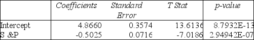Note: 2.94942E-07 = 2.94942*10⁻⁷ -Referring to Table 13-7, to test whether the prison stocks portfolio is negatively related to the S&P 500 index, the measured value of the test statistic is

TABLE 13-11 A computer software developer would like to use the number of downloads (in thousands) for the trial version of his new shareware to predict the amount of revenue (in thousands of dollars) he can make on the full version of the new shareware. 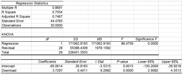Following is the output from a simple linear regression along with the residual plot and normal probability plot obtained from a data set of 30 different sharewares that he has developed: -Referring to Table 13-11, which of the following is the correct null hypothesis for testing whether there is a linear relationship between revenue and the number of downloads?

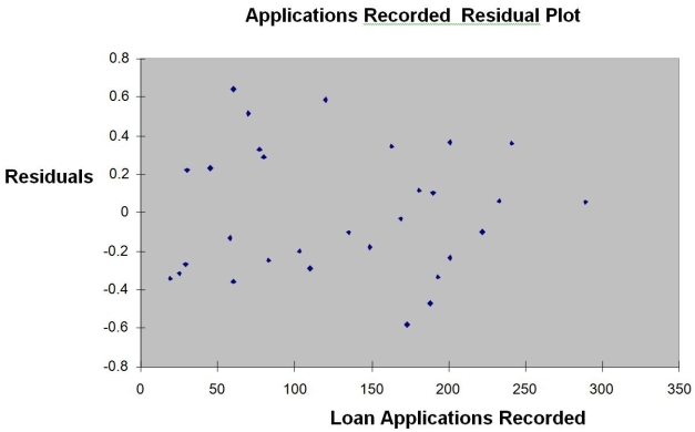
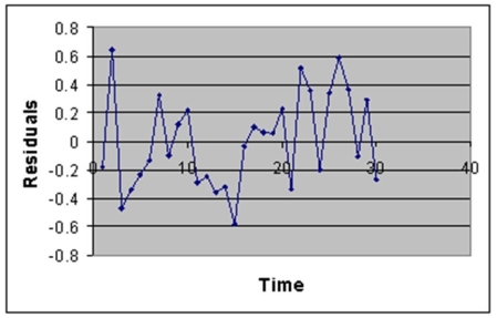
TABLE 13-12 The manager of the purchasing department of a large saving and loan organization would like to develop a model to predict the amount of time (measured in hours) it takes to record a loan application. Data are collected from a sample of 30 days, and the number of applications recorded and completion time in hours is recorded. Below is the regression output: 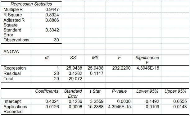Note: 4.3946E-15 is 4.3946 × -Referring to Table 13-12, the degrees of freedom for the F test on whether the number of load applications recorded affects the amount of time are

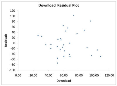
TABLE 13-11 A computer software developer would like to use the number of downloads (in thousands) for the trial version of his new shareware to predict the amount of revenue (in thousands of dollars) he can make on the full version of the new shareware. Following is the output from a simple linear regression along with the residual plot and normal probability plot obtained from a data set of 30 different sharewares that he has developed: -Referring to Table 13-11, there appears to be autocorrelation in the residuals.

When r = -1, it indicates a perfect relationship between X and Y.

TABLE 13-10 The management of a chain electronic store would like to develop a model for predicting the weekly sales (in thousands of dollars) for individual stores based on the number of customers who made purchases. A random sample of 12 stores yields the following results: -Referring to Table 13-10, the mean weekly sales will increase by an estimated $10 for each additional purchasing customer.

TABLE 13-3 The director of cooperative education at a state college wants to examine the effect of cooperative education job experience on marketability in the work place. She takes a random sample of 4 students. For these 4, she finds out how many times each had a cooperative education job and how many job offers they received upon graduation. These data are presented in the table below. 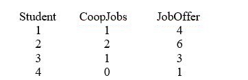-Referring to Table 13-3, the coefficient of determination is ________.

TABLE 13-10 The management of a chain electronic store would like to develop a model for predicting the weekly sales (in thousands of dollars) for individual stores based on the number of customers who made purchases. A random sample of 12 stores yields the following results: -Referring to Table 13-10, what is the p-value of the F test statistic when testing whether the number of customers who make purchases is a good predictor for weekly sales?

TABLE 13-3 The director of cooperative education at a state college wants to examine the effect of cooperative education job experience on marketability in the work place. She takes a random sample of 4 students. For these 4, she finds out how many times each had a cooperative education job and how many job offers they received upon graduation. These data are presented in the table below. -Referring to Table 13-3, the error or residual sum of squares (SSE) is ________.

TABLE 13-10 The management of a chain electronic store would like to develop a model for predicting the weekly sales (in thousands of dollars) for individual stores based on the number of customers who made purchases. A random sample of 12 stores yields the following results: -Referring to Table 13-10, what is the value of the coefficient of correlation?

TABLE 13-5 The managing partner of an advertising agency believes that his company's sales are related to the industry sales. He uses Microsoft Excel to analyze the last 4 years of quarterly data (i.e., n = 16) with the following results: 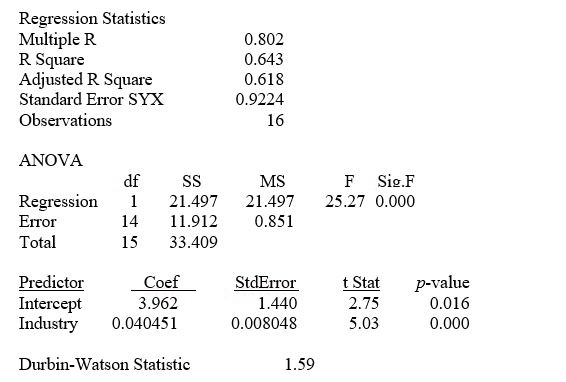-Referring to Table 13-5, the estimates of the Y-intercept and slope are ________ and ________, respectively.

TABLE 13-9 It is believed that, the average numbers of hours spent studying per day (HOURS) during undergraduate education should have a positive linear relationship with the starting salary (SALARY, measured in thousands of dollars per month) after graduation. Given below is the Excel output for predicting starting salary (Y) using number of hours spent studying per day (X) for a sample of 51 students. NOTE: Only partial output is shown. 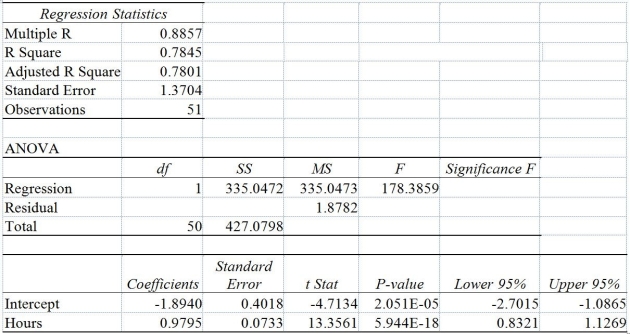Note: 2.051E - 05 = 2.051*10⁻⁰⁵ and 5.944E - 18 = 5.944*10⁻¹⁸. -Referring to Table 13-9, to test the claim that SALARY depends positively on HOURS against the null hypothesis that SALARY does not depend linearly on HOURS, the p-value of the test statistic is

Referring to Table 13-2, if the price of the candy bar is set at $2, the estimated mean sales will be

TABLE 13-10 The management of a chain electronic store would like to develop a model for predicting the weekly sales (in thousands of dollars) for individual stores based on the number of customers who made purchases. A random sample of 12 stores yields the following results: -Referring to Table 13-10, the value of the t test statistic and F test statistic should be the same when testing whether the number of customers who make purchases is a good predictor for weekly sales.

TABLE 13-12 The manager of the purchasing department of a large saving and loan organization would like to develop a model to predict the amount of time (measured in hours) it takes to record a loan application. Data are collected from a sample of 30 days, and the number of applications recorded and completion time in hours is recorded. Below is the regression output: Note: 4.3946E-15 is 4.3946 × -Referring to Table 13-12, there is sufficient evidence that the amount of time needed linearly depends on the number of loan applications at a 5% level of significance.

TABLE 13-4 The managers of a brokerage firm are interested in finding out if the number of new clients a broker brings into the firm affects the sales generated by the broker. They sample 12 brokers and determine the number of new clients they have enrolled in the last year and their sales amounts in thousands of dollars. These data are presented in the table that follows. 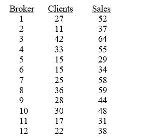-Referring to Table 13-4, the managers of the brokerage firm wanted to test the hypothesis that the population slope was equal to 0. The p-value of the test is ________.

TABLE 13-12 The manager of the purchasing department of a large saving and loan organization would like to develop a model to predict the amount of time (measured in hours) it takes to record a loan application. Data are collected from a sample of 30 days, and the number of applications recorded and completion time in hours is recorded. Below is the regression output: Note: 4.3946E-15 is 4.3946 × -Referring to Table 13-12, there is a 95% probability that the mean amount of time needed to record one additional loan application is somewhere between 0.0109 and 0.0143 hours.

TABLE 13-13 In this era of tough economic conditions, voters increasingly ask the question: "Is the educational achievement level of students dependent on the amount of money the state in which they reside spends on education?" The partial computer output below is the result of using spending per student ($) as the independent variable and composite score which is the sum of the math, science and reading scores as the dependent variable on 35 states that participated in a study. The table includes only partial results. 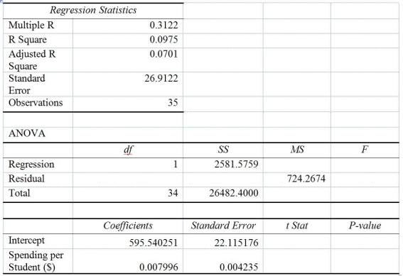-Referring to Table 13-13, what is the standard deviation of the composite score around the regression line?

TABLE 13-12 The manager of the purchasing department of a large saving and loan organization would like to develop a model to predict the amount of time (measured in hours) it takes to record a loan application. Data are collected from a sample of 30 days, and the number of applications recorded and completion time in hours is recorded. Below is the regression output: Note: 4.3946E-15 is 4.3946 × -Referring to Table 13-12, the model appears to be adequate based on the residual analyses.

TABLE 13-4 The managers of a brokerage firm are interested in finding out if the number of new clients a broker brings into the firm affects the sales generated by the broker. They sample 12 brokers and determine the number of new clients they have enrolled in the last year and their sales amounts in thousands of dollars. These data are presented in the table that follows. -Referring to Table 13-4, the managers of the brokerage firm wanted to test the hypothesis that the population slope was equal to 0. At a level of significance of 0.01, the null hypothesis should be ________ (rejected or not rejected).