Exam 7: Comparing Two Means

In order to investigate whether talking on cell phones is more distracting than listening to car radios while driving, sixty-four student volunteers (from a single college class) were randomly assigned to a cell phone group or a radio group (32 students were assigned to each group). Each student "drove" a machine that simulated driving situations. While "driving" the simulator, a target would flash red at irregular intervals. Participants were instructed to press the "brake" button as soon as possible when they detected a red light. Participant response times were measured as the time between the red light appearing and pushing the brake button. While driving, the radio group listened to a radio broadcast and the cell phone group carried on a conversation on the cell phone with someone in the next room. The cell phone group had an average response time of 585.2 milliseconds (SD = 89.6), and the control group had an average response time of 533.7 milliseconds (SD = 65.3). -Use the Theory-Based Inference applet to find the theory-based p-value to determine whether talking on cell phones is more distracting than listening to the radio while driving.

Do children diagnosed with attention deficit/hyperactivity disorder (ADHD) have smaller brains than children without this condition? Brain scans were completed for 152 children with ADHD and 139 children of similar age without ADHD. The mean brain size for the 152 children with ADHD was 1059.4 mL with a standard deviation of 117.5 mL. The mean brain size for the 139 children of with-out ADHD was 1104.5 mL with a standard deviation of 111.3 mL. -How could you simulate one sample under the null hypothesis?

Monthly snowfall (in inches) was measured over several winters in Fort Collins, Colorado. Researchers also recorded whether the measurement was taken in the Early winter (September to December) or Late winter (January to June). Boxplots displaying the distribution of monthly snowfall for each season are below. 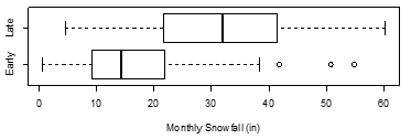-Which season has the larger inter-quartile range (IQR) of monthly snowfall?

What would the appropriate hypotheses be in order to investigate whether college upperclassmen tend to spend less on textbooks than college underclassmen?

The plot below displays the on-base percentage for all Major League Baseball players who played in at least 15 games during the 2018 MLB season based on the player's position. Positions: 1/2/3B = 1st/2nd/3rd base, C = catcher, C/L/RF = center/left/right field, DH = designated hitter, P = pitcher, SS = short stop On-base percentage = (hits + walks + hit by pitch)/(total plate appearances) 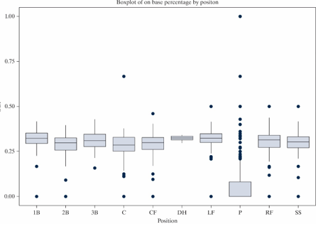-Which of the positions has the smallest inter-quartile range (IQR) of on-base percentages?

An article that appeared in the British Medical Journal (2010) presented the results of a randomized experiment conducted by researcher Jeremy Groves, whose objective was to determine whether the weight of his bicycle could affect his travel time to work. On each of 56 days (from mid-January to mid-July 2010), Groves tossed a £1 coin to decide whether he would be biking to work on his carbon frame (lighter) bicycle that weighed 20.9 lbs or on his steel frame (heavier) bicycle that weighed 29.75 lbs. He then recorded the commute time (in minutes) for each trip. Here are the summary statistics for his data: 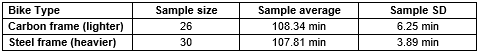-The p-value comparing the two average commute times for the two different bikes was found to be 0.728. Which of the following is the most appropriate conclusion based on this p-value?