Exam 13: Regression and Forecasting Models

Exhibit 13-1 An express delivery service company recently conducted a study to investigate the relationship between the cost of shipping a package (Y), the package weight in pounds (X₁), and the distance shipped in miles (X₂). Twenty packages were randomly selected from among the large number received for shipment, and a detailed analysis of the shipping cost was conducted for each package. The sample information is shown in the table below: Cost of Shipment Package Weight Distance Shi \ 3.40 4.3 100 \ 2.10 0.5 165 \ 11.10 5.3 245 \ 2.70 6.1 52 \ 2.00 4.7 58 \ 8.10 3.7 255 \ 15.60 7.2 265 \ 5.10 2.6 214 \ 1.10 0.8 105 \ 4.50 0.95 285 \ 6.10 6.4 120 \ 1.80 1.3 95 \ 14.60 6.7 245 \ 14.10 7.7 195 \ 9.30 6.8 165 \ 1.20 2.9 50 \ 12.20 8.3 165 \ 1.60 0.9 85 \ 8.10 4.6 207 \ 4.00 3.4 150 -Refer to Exhibit 13-1.How does the R² value for this multiple regression model compare to that of the simple regression model estimated above Interpret the adjusted R² values for the two models.

Exhibit 13-1 An express delivery service company recently conducted a study to investigate the relationship between the cost of shipping a package (Y), the package weight in pounds (X₁), and the distance shipped in miles (X₂). Twenty packages were randomly selected from among the large number received for shipment, and a detailed analysis of the shipping cost was conducted for each package. The sample information is shown in the table below: Cost of Shipment Package Weight Distance Shi \ 3.40 4.3 100 \ 2.10 0.5 165 \ 11.10 5.3 245 \ 2.70 6.1 52 \ 2.00 4.7 58 \ 8.10 3.7 255 \ 15.60 7.2 265 \ 5.10 2.6 214 \ 1.10 0.8 105 \ 4.50 0.95 285 \ 6.10 6.4 120 \ 1.80 1.3 95 \ 14.60 6.7 245 \ 14.10 7.7 195 \ 9.30 6.8 165 \ 1.20 2.9 50 \ 12.20 8.3 165 \ 1.60 0.9 85 \ 8.10 4.6 207 \ 4.00 3.4 150 -Refer to Exhibit 13-1.Add the second explanatory variable (distance shipped)to the regression model.Estimate and interpret the slopes of this expanded model.

Exhibit 13-3 The quarterly numbers of applications for home mortgage loans at a branch office of a large bank are recorded in the table below. 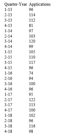-Refer to Exhibit 13-3.Obtain a simple exponential smoothing forecast again,this time optimizing the smoothing constant.Does it make much of an improvement

Exhibit 13-1 An express delivery service company recently conducted a study to investigate the relationship between the cost of shipping a package (Y), the package weight in pounds (X₁), and the distance shipped in miles (X₂). Twenty packages were randomly selected from among the large number received for shipment, and a detailed analysis of the shipping cost was conducted for each package. The sample information is shown in the table below: Cost of Shipment Package Weight Distance Shi \ 3.40 4.3 100 \ 2.10 0.5 165 \ 11.10 5.3 245 \ 2.70 6.1 52 \ 2.00 4.7 58 \ 8.10 3.7 255 \ 15.60 7.2 265 \ 5.10 2.6 214 \ 1.10 0.8 105 \ 4.50 0.95 285 \ 6.10 6.4 120 \ 1.80 1.3 95 \ 14.60 6.7 245 \ 14.10 7.7 195 \ 9.30 6.8 165 \ 1.20 2.9 50 \ 12.20 8.3 165 \ 1.60 0.9 85 \ 8.10 4.6 207 \ 4.00 3.4 150 -Refer to Exhibit 13-1.Estimate a simple linear regression model involving shipping cost and package weight.Interpret the slope coefficient of the least squares line as well as R².

Forecasting models can be divided into three groups.They are:

Winter's method is an exponential smoothing method,which is appropriate for a series with trend but no seasonality.

Exhibit 13-3 The quarterly numbers of applications for home mortgage loans at a branch office of a large bank are recorded in the table below. -Refer to Exhibit 13-3.Use a moving average model to forecast these data,requesting 4 quarters of future forecasts.Use a span of 4 quarters.

The least squares line is the line that minimizes the sum of the residuals.

Which of the following is not one of the commonly used summary measures for forecast errors

Exhibit 13-3 The quarterly numbers of applications for home mortgage loans at a branch office of a large bank are recorded in the table below. -Refer to Exhibit 13-3.Use simple exponential smoothing to forecast these data,requesting 4 quarters of future forecasts.Use the default smoothing constant of 0.10.Is this better than the moving average model