Exam 12: Simple Linear Regression
Exam 1: Defining and Collecting Data145 Questions
Exam 2: Organising and Visualising Data203 Questions
Exam 3: Numerical Descriptive Measures147 Questions
Exam 4: Basic Probability168 Questions
Exam 5: Some Important Discrete Probability Distributions172 Questions
Exam 6: The Normal Distribution and Other Continuous Distributions190 Questions
Exam 7: Sampling Distributions133 Questions
Exam 8: Confidence Interval Estimation186 Questions
Exam 9: Fundamentals of Hypothesis Testing: One-Sample Tests180 Questions
Exam 10: Hypothesis Testing: Two-Sample Tests175 Questions
Exam 11: Analysis of Variance148 Questions
Exam 12: Simple Linear Regression207 Questions
Exam 13: Introduction to Multiple Regression269 Questions
Exam 14: Time-Series Forecasting and Index Numbers201 Questions
Exam 15: Chi-Square Tests134 Questions
Exam 16: Multiple Regression Model Building93 Questions
Exam 17: Decision Making106 Questions
Exam 18: Statistical Applications in Quality Management119 Questions
Exam 19: Further Non-Parametric Tests50 Questions
Select questions type
What do we mean when we say that a simple linear regression model is 'statistically' useful?
(Multiple Choice)
4.8/5  (31)
(31)
Instruction 12.8
It is believed that the average numbers of hours spent studying per day (HOURS) during undergraduate education should have a positive linear relationship with the starting salary (SALARY, measured in thousands of dollars per month) after graduation. Given below is the Microsoft Excel output for predicting starting salary (Y) using number of hours spent studying per day (X) for a sample of 51 students. NOTE: Only partial output is shown.
MultipleR 0.8857 R Square 0.7845 Adjusted R Square 0.7801 Standard Error 1.3704 Observations 51
ANOVA df 55 MS F Significance F Regression 1 335.0472 335.0473 178.3859 Residual 1.8782 Total 50 427.0798
Coefficients Standard Error tStat p-value Lower 95\% Upper 95\% Intercept -1.8940 0.4018 -4.7134 2.051-05 -2.7015 -1.0865 Hours 0.9795 0.0733 13.3561 5.944-18 0.8321 1.1269 Note: 2.051E-05 = 2.051 * 10S1-0.5 and 5.944E-18 = 5.944 * 10S1-18.
-Referring to Instruction 12.8,the error sum of squares (SSE)of the above regression is
(Multiple Choice)
4.9/5 (36)
Instruction 12.14
The managing partner of an advertising agency believes that his company's sales are related to the industry sales. He uses Microsoft Excel's Data Analysis tool to analyse the last four years of quarterly data with the following results:
Multiple R 0.802 R Square 0.643 Adjusted R Square 0.618 Standard Error SYX 0.9224 Observations 16
df SS MS F Sig.F Regression 1 21.497 21.497 25.27 0.000 Error 14 11.912 0.851 Total 15 33.409
Predictor Coef StdError t Stat p-value Intercept 3.962 1.440 2.75 0.016 Industry 0.040451 0.008048 5.03 0.000
Durbin-Watson 1.59 Statistic
-Referring to Instruction 12.14,the correlation coefficient is ____________.
(Short Answer)
4.7/5 (37)
The sample correlation coefficient between X and Y is 0.375.It has been found out that the p-value is 0.256 when testing H0: ρ = 0 against the two-sided alternative H1: ρ ≠ 0.To test H0: ρ = 0 against the one-sided alternative H1: ρ > 0 at a significance level of 0.2,the p-value is
(Multiple Choice)
5.0/5 (32)
Instruction 12.23
The managing partner of an advertising agency believes that his company's sales are related to the industry sales. He uses Microsoft Excel's Data Analysis tool to analyse the last four years of quarterly data with the following results:
Multiple R 0.802 R Square 0.643 Adjusted R Square 0.618 Standard Error SYX 0.9224 Observations 16
df SS MS F Sig.F Regression 1 21.497 21.497 25.27 0.000 Error 14 11.912 0.851 Total 15 33.409
Predictor Coef StdError t Stat p-value Intercept 3.962 1.440 2.75 0.016 Industry 0.040451 0.008048 5.03 0.000
Durbin-Watson 1.59 Statistic
-Referring to Instruction 12.23,the partner wants to test for autocorrelation using the Durbin-Watson statistic.Using a level of significance of 0.05,the decision he should make is
(Multiple Choice)
4.7/5 (33)
onfident that the mean amount of time needed to record one additional loan application is somewhere
MultipleR 0.9447 R Square 0.8924 Adjusted R Square 0.8886 Standard Error 0.3342 Observations 30
df S5 MS F Significance F Regression 1 25.9438 25.9438 232.2200 4.3946-15 Residual 28 3.1282 0.1117 Total 29 29.072
Coefficients Standard Error tStat p-value Lower 95\% Upper 95\% Intercept 0.4024 0.1236 3.2559 0.0030 0.1492 0.6555 Applications Recorded 0.0126 0.0008 15.2388 4.3946- 15 0.0109 0.0143
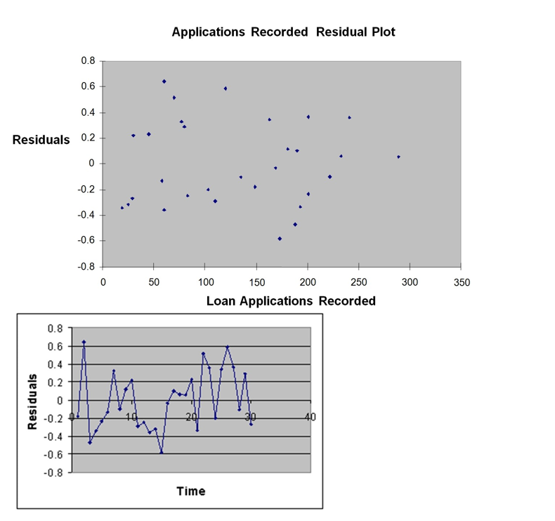 -Referring to Instruction 12.36,there is a 95% probability that the mean amount of time needed to record one additional loan application is somewhere between 0.0109 and 0.0143 hours.
(True/False)
4.8/5 (30)
Instruction 12.2
A chocolate bar manufacturer is interested in trying to estimate how sales are influenced by the price of their product. To do this, the company randomly chooses six country towns and cities and offers the chocolate bar at different prices. Using chocolate bar sales as the dependent variable, the company will conduct a simple linear regression on the data below:
-Referring to Instruction 12.2,what is the standard error of the regression slope estimate, ?
(Multiple Choice)
4.8/5 (31)
Based on the residual plot below,you will conclude that there might be a violation of which of the following assumptions? 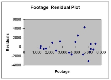
(Multiple Choice)
4.7/5 (30)
Instruction 12.35
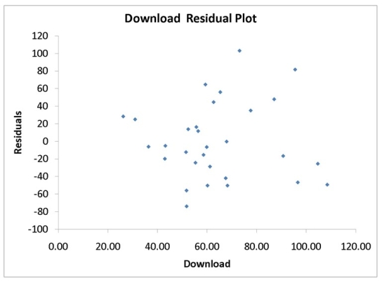
A computer software developer would like to use the number of downloads (in thousands) for the trial version of his new shareware to predict the amount of revenue (in thousands of dollars) he can make on the full version of the new shareware. Following is the output from a simple linear regression along with the residual plot and normal probability plot obtained from a data set of 30 different sharewares that he has developed:
MultipleR 0.8691 R Square 0.7554 Adjusted R Square 0.7467 Standard Error 44.4765 Observations 30.0000
df SS MS F Significance F Regression 1 171062.9193 171062.9193 86.4759 0.0000 Residual 28 55388.4309 1978.1582 Total 29 226451.3503
Coefficients Standard Error t Stat p -value Lower 95\% Upper 95\% Intercept -95.0614 26.9183 -3.5315 0.0015 -150.2009 -39.9218 Download 3.7297 0.4011 9.2992 0.0000 2.9082 4.5513
 -Referring to Instruction 12.35,which of the following is the correct alternative hypothesis for testing whether there is a linear relationship between revenue and number of downloads?
(Multiple Choice)
4.8/5 (38)
Instruction 12.3
The director of cooperative education at a university wants to examine the effect of cooperative education job experience on marketability in the workplace. She takes a random sample of four students. For these four, she finds out how many times each had a cooperative education job and how many job offers they received upon graduation. These data are presented in the table below.
Student Coop jobs job Offer 1 1 4 2 2 6 3 1 3 4 0 1
-Referring to Instruction 12.3,the regression sum of squares (SSR)is____________.
(Short Answer)
4.8/5 (36)
Instruction 12.38
The director of cooperative education at a university wants to examine the effect of cooperative education job experience on marketability in the workplace. She takes a random sample of four students. For these four, she finds out how many times each had a cooperative education job and how many job offers they received upon graduation. These data are presented in the table below.
Student Coop Jobs Job Oifer 1 1 4 2 2 6 3 1 3 4 0 1
-Referring to Instruction 12.38,suppose the director of cooperative education wants to obtain a 95% confidence-interval estimate for the mean number of job offers received by students who have had exactly one cooperative education job.The t critical value she would use is_____________.
(Short Answer)
4.9/5 (22)
The width of the prediction interval for the predicted value of Y is dependent on
(Multiple Choice)
4.9/5 (30)
Instruction 12.38
The director of cooperative education at a university wants to examine the effect of cooperative education job experience on marketability in the workplace. She takes a random sample of four students. For these four, she finds out how many times each had a cooperative education job and how many job offers they received upon graduation. These data are presented in the table below.
Student Coop Jobs Job Oifer 1 1 4 2 2 6 3 1 3 4 0 1
-Referring to Instruction 12.38,suppose the director of cooperative education wants to construct a 95% prediction interval for the number of job offers received by a student who has had exactly two cooperative education jobs.The prediction interval is from __________ to __________.
(Short Answer)
4.9/5 (34)
Instruction 12.34
The management of a chain electronic store would like to develop a model for predicting the weekly sales (in thousands of dollars) for individual stores based on the number of customers who made purchases. A random sample of 12 stores yields the following results:
Customers Sales (Thousands of Dollars) 907 11.20 926 11.05 713 8.21 741 9.21 780 9.42 898 10.08 510 6.73 529 7.02 460 6.12 872 9.52 650 7.53 603 7.25
-Referring to Instruction 12.34,the average weekly sales will increase by an estimated $0.01 for each additional purchasing customer.
(True/False)
4.7/5 (31)
Instruction 12.27
The director of cooperative education at a university wants to examine the effect of cooperative education job experience on marketability in the workplace. She takes a random sample of four students. For these four, she finds out how many times each had a cooperative education job and how many job offers they received upon graduation. These data are presented in the table below.
Student Coop jobs job Offer 1 1 4 2 2 6 3 1 3 4 0 1
-Referring to Instruction 12.27,the director of cooperative education wanted to test the hypothesis that the true slope was equal to 0.The denominator of the test statistic is .The value of in this sample is____________
(Short Answer)
4.9/5 (25)
Instruction 12.19
A computer software developer would like to use the number of downloads (in thousands) for the trial version of his new shareware to predict the amount of revenue (in thousands of dollars) he can make on the full version of the new shareware. Following is the output from a simple linear regression along with the residual plot and normal probability plot obtained from a data set of 30 different sharewares that he has developed:
MultipleR 0.8691 R Square 0.7554 Adjusted R Square 0.7467 Standard Error 44.4765 Observations 30.0000
df SS MS F Significance F Regression 1 171062.9193 171062.9193 86.4759 0.0000 Residual 28 55388.4309 1978.1582 Total 29 226451.3503
Coefficients Standard Error t Stat p -value Lower 95\% Upper 95\% Intercept -95.0614 26.9183 -3.5315 0.0015 -150.2009 -39.9218 Download 3.7297 0.4011 9.2992 0.0000 2.9082 4.5513

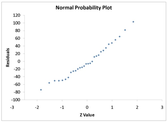 -Referring to Instruction 12.19,which of the following assumptions appears to have been violated?
(Multiple Choice)
4.9/5 (29)
Instruction 12.31
An investment specialist claims that if one holds a portfolio that moves in opposite direction to the market index like the All Ordinaries Index, then it is possible to reduce the variability of the portfolio's return. In other words, one can create a portfolio with positive returns but less exposure to risk. A sample of 26 years of the All Ordinaries index and a portfolio consisting of stocks of private prisons, which are believed to be negatively related to the All Ordinaries index, is collected. A regression analysis was performed by regressing the returns of the prison stocks portfolio (Y) on the returns of All Ordinaries index (X) to prove that the prison stocks portfolio is negatively related to the All Ordinaries index at a 5% level of significance. The results are given in the following Microsoft Excel output.
Coefflelents Standard Error tStat p -vahse Intercept 4.866004258 0.35743609 13.61363441 8.7932-13 S\&P -0.502513506 0.071597152 -7.01862425 2.94942-07
-Referring to Instruction 12.31,to test whether the prison stocks portfolio is negatively related to the All Ordinaries index,the p-value of the associated test statistic is
(Multiple Choice)
4.7/5 (32)
Instruction 12.25
A computer software developer would like to use the number of downloads (in thousands) for the trial version of his new shareware to predict the amount of revenue (in thousands of dollars) he can make on the full version of the new shareware. Following is the output from a simple linear regression along with the residual plot and normal probability plot obtained from a data set of 30 different sharewares that he has developed:
MultipleR 0.8691 R Square 0.7554 Adjusted R Square 0.7467 Standard Error 44.4765 Observations 30.0000
df SS MS F Significance F Regression 1 171062.9193 171062.9193 86.4759 0.0000 Residual 28 55388.4309 1978.1582 Total 29 226451.3503
Coefficients Standard Error t Stat p -value Lower 95\% Upper 95\% Intercept -95.0614 26.9183 -3.5315 0.0015 -150.2009 -39.9218 Download 3.7297 0.4011 9.2992 0.0000 2.9082 4.5513

 -Referring to Instruction 12.25,the Durbin-Watson statistic is inappropriate for this data set.
(Essay)
4.7/5 (36)
Instruction 12.35
A computer software developer would like to use the number of downloads (in thousands) for the trial version of his new shareware to predict the amount of revenue (in thousands of dollars) he can make on the full version of the new shareware. Following is the output from a simple linear regression along with the residual plot and normal probability plot obtained from a data set of 30 different sharewares that he has developed:
MultipleR 0.8691 R Square 0.7554 Adjusted R Square 0.7467 Standard Error 44.4765 Observations 30.0000
df SS MS F Significance F Regression 1 171062.9193 171062.9193 86.4759 0.0000 Residual 28 55388.4309 1978.1582 Total 29 226451.3503
Coefficients Standard Error t Stat p -value Lower 95\% Upper 95\% Intercept -95.0614 26.9183 -3.5315 0.0015 -150.2009 -39.9218 Download 3.7297 0.4011 9.2992 0.0000 2.9082 4.5513
-Referring to Instruction 12.35,what is the p-value for testing whether there is a linear relationship between revenue and the number of downloads at a 5% level of significance?
(Short Answer)
4.9/5 (40)
Instruction 12.23
The managing partner of an advertising agency believes that his company's sales are related to the industry sales. He uses Microsoft Excel's Data Analysis tool to analyse the last four years of quarterly data with the following results:
Multiple R 0.802 R Square 0.643 Adjusted R Square 0.618 Standard Error SYX 0.9224 Observations 16
df SS MS F Sig.F Regression 1 21.497 21.497 25.27 0.000 Error 14 11.912 0.851 Total 15 33.409
Predictor Coef StdError t Stat p-value Intercept 3.962 1.440 2.75 0.016 Industry 0.040451 0.008048 5.03 0.000
Durbin-Watson 1.59 Statistic
-Referring to Instruction 12.23,if the Durbin-Watson statistic has a value close to 4,which assumption is violated?
(Multiple Choice)
4.9/5 (35)
Filters
- Essay(0)
- Multiple Choice(0)
- Short Answer(0)
- True False(0)
- Matching(0)