Exam 12: Simple Linear Regression
Exam 1: Defining and Collecting Data145 Questions
Exam 2: Organising and Visualising Data203 Questions
Exam 3: Numerical Descriptive Measures147 Questions
Exam 4: Basic Probability168 Questions
Exam 5: Some Important Discrete Probability Distributions172 Questions
Exam 6: The Normal Distribution and Other Continuous Distributions190 Questions
Exam 7: Sampling Distributions133 Questions
Exam 8: Confidence Interval Estimation186 Questions
Exam 9: Fundamentals of Hypothesis Testing: One-Sample Tests180 Questions
Exam 10: Hypothesis Testing: Two-Sample Tests175 Questions
Exam 11: Analysis of Variance148 Questions
Exam 12: Simple Linear Regression207 Questions
Exam 13: Introduction to Multiple Regression269 Questions
Exam 14: Time-Series Forecasting and Index Numbers201 Questions
Exam 15: Chi-Square Tests134 Questions
Exam 16: Multiple Regression Model Building93 Questions
Exam 17: Decision Making106 Questions
Exam 18: Statistical Applications in Quality Management119 Questions
Exam 19: Further Non-Parametric Tests50 Questions
Select questions type
Instruction 12.35
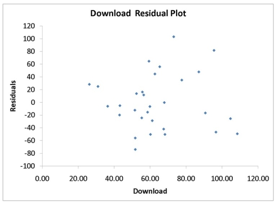
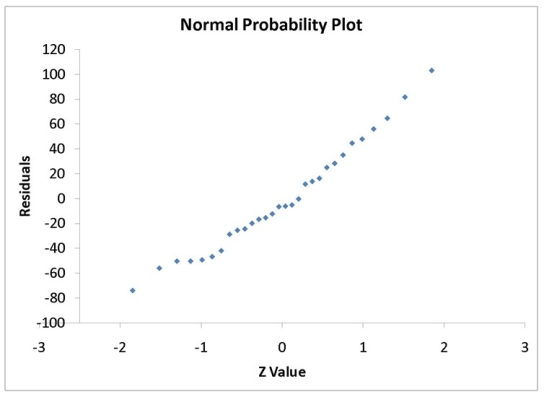
A computer software developer would like to use the number of downloads (in thousands) for the trial version of his new shareware to predict the amount of revenue (in thousands of dollars) he can make on the full version of the new shareware. Following is the output from a simple linear regression along with the residual plot and normal probability plot obtained from a data set of 30 different sharewares that he has developed:
MultipleR 0.8691 R Square 0.7554 Adjusted R Square 0.7467 Standard Error 44.4765 Observations 30.0000
df SS MS F Significance F Regression 1 171062.9193 171062.9193 86.4759 0.0000 Residual 28 55388.4309 1978.1582 Total 29 226451.3503
Coefficients Standard Error t Stat p -value Lower 95\% Upper 95\% Intercept -95.0614 26.9183 -3.5315 0.0015 -150.2009 -39.9218 Download 3.7297 0.4011 9.2992 0.0000 2.9082 4.5513
 -Referring to Instruction 12.35,there is sufficient evidence that revenue and number of downloads are linearly related at a 5% level of significance.
(True/False)
4.8/5  (32)
(32)
A zero population correlation coefficient between a pair of random variables means that there is no linear relationship between the random variables.
(True/False)
4.8/5 (33)
onfident that the mean amount of time needed to record one additional loan application is somewhere
MultipleR 0.9447 R Square 0.8924 Adjusted R Square 0.8886 Standard Error 0.3342 Observations 30
df S5 MS F Significance F Regression 1 25.9438 25.9438 232.2200 4.3946-15 Residual 28 3.1282 0.1117 Total 29 29.072
Coefficients Standard Error tStat p-value Lower 95\% Upper 95\% Intercept 0.4024 0.1236 3.2559 0.0030 0.1492 0.6555 Applications Recorded 0.0126 0.0008 15.2388 4.3946- 15 0.0109 0.0143
 -Referring to Instruction 12.36,the value of the measured t test statistic to test whether the amount of time depends linearly on the number of loan applications recorded is
(Multiple Choice)
4.9/5 (35)
Instruction 12.33
It is believed that the average numbers of hours spent studying per day (HOURS) during undergraduate education should have a positive linear relationship with the starting salary (SALARY, measured in thousands of dollars per month) after graduation. Given below is the Microsoft Excel output for predicting starting salary (Y) using number of hours spent studying per day (X) for a sample of 51 students. NOTE: Only partial output is shown.
Multiple R 0.8857 R Square 0.7845 Adjusted R Square 0.7801 Standard Error 1.3704 Observations 51
df SS MS F Significance F Regression 1 335.0472 335.0473 178.3859 Residual 1.8782 Total 50 427.0798
Coefficients Standard Error t Stat p-value Lower 95\% Upper 95\% Intercept -1.8940 0.4018 -4.7134 2.051-05 -2.7015 -1.0865 Hours 0.9795 0.0733 13.3561 5.944-18 0.8321 1.1269 Note: 2.051E-05 = 2.051 * 10-0.5 and 5.944E-18 = 5.944 * 10-18.
-Referring to Instruction 12.33,the value of the measured t test statistic to test whether average SALARY depends linearly on HOURS is
(Multiple Choice)
4.8/5 (36)
A simple regression has a b0 value of 5 and a b1 value of 3.5.What is the predicted Y for an X value of -2?
(Multiple Choice)
4.9/5 (38)
Instruction 12.29
The managers of a brokerage firm are interested in finding out if the number of new customers a broker brings into the firm affects the sales generated by the broker. They sample 12 brokers and determine the number of new customers they have enrolled in the last year and their sales amounts in thousands of dollars. These data are presented in the table that follows.
Broker Clients Sales 1 27 52 2 11 37 3 42 64 4 33 55 5 15 29 6 15 34 7 25 58 8 36 59 9 28 44 10 30 48 11 17 31 12 22 38
-Referring to Instruction 12.29,the managers of the brokerage firm wanted to test the hypothesis that the number of new customers brought in had a positive impact on the amount of sales generated.The value of the test statistic is ____________
(Short Answer)
4.8/5 (40)
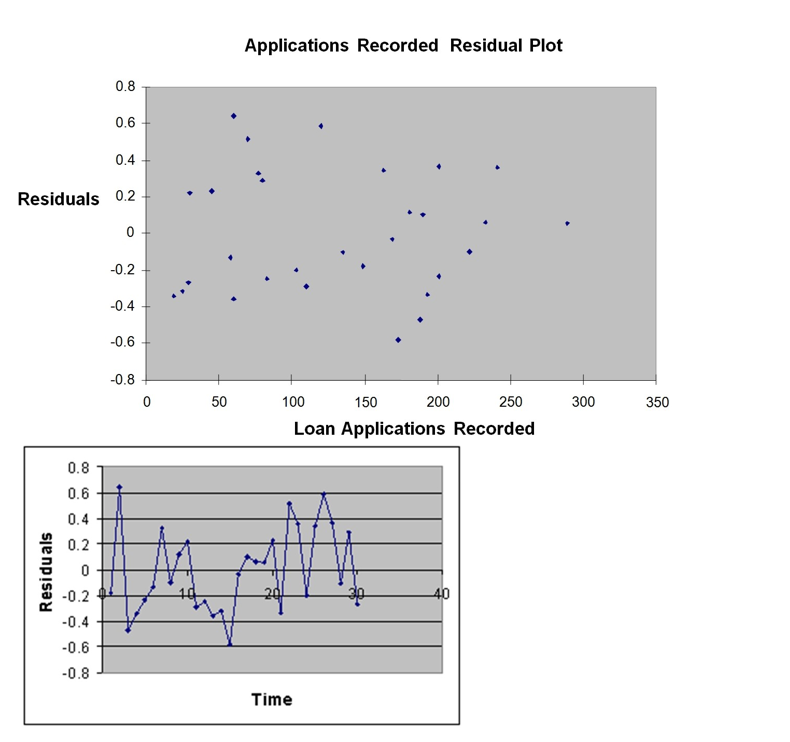
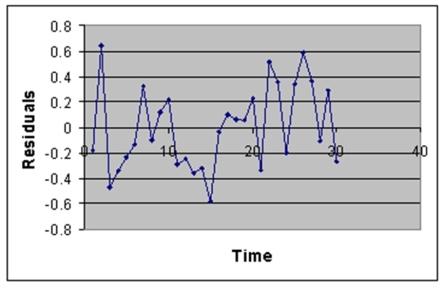
To determine whether the linear model is appropriate and to check the equal variance assumption,plot residuals against the independent variable.
(True/False)
4.8/5 (28)
onfident that the mean amount of time needed to record one additional loan application is somewhere
MultipleR 0.9447 R Square 0.8924 Adjusted R Square 0.8886 Standard Error 0.3342 Observations 30
df S5 MS F Significance F Regression 1 25.9438 25.9438 232.2200 4.3946-15 Residual 28 3.1282 0.1117 Total 29 29.072
Coefficients Standard Error tStat p-value Lower 95\% Upper 95\% Intercept 0.4024 0.1236 3.2559 0.0030 0.1492 0.6555 Applications Recorded 0.0126 0.0008 15.2388 4.3946- 15 0.0109 0.0143
-Referring to Instruction 12.36,the 90% confidence interval for the mean change in the amount of time needed as a result of recording one additional loan application is
(Multiple Choice)
4.7/5 (38)
Instruction 12.17
A computer software developer would like to use the number of downloads (in thousands) for the trial version of his new shareware to predict the amount of revenue (in thousands of dollars) he can make on the full version of the new shareware. Following is the output from a simple linear regression along with the residual plot and normal probability plot obtained from a data set of 30 different sharewares that he has developed:
MultipleR 0.8691 R Square 0.7554 Adjusted R Square 0.7467 Standard Error 44.4765 Observations 30.0000
df SS MS F Significance F Regression 1 171062.9193 171062.9193 86.4759 0.0000 Residual 28 55388.4309 1978.1582 Total 29 226451.3503
Coefficients Standard Error t Stat p -value Lower 95\% Upper 95\% Intercept -95.0614 26.9183 -3.5315 0.0015 -150.2009 -39.9218 Download 3.7297 0.4011 9.2992 0.0000 2.9082 4.5513

 -Referring to Instruction 12.17,what is the standard error of estimate?
(Short Answer)
4.7/5 (37)
Which of the following can be used to check the normality assumption?
(Multiple Choice)
4.7/5 (42)
Instruction 12.9
The management of a chain electronic store would like to develop a model for predicting the weekly sales (in thousands of dollars) for individual stores based on the number of customers who made purchases. A random sample of 12 stores yields the following results:
Customers Sales (Thousands of Dollars) 907 11.20 926 11.05 713 8.21 741 9.21 780 9.42 898 10.08 510 6.73 529 7.02 460 6.12 872 9.52 650 7.53 603 7.25
-Referring to Instruction 12.9,93.98% of the total variation in weekly sales can be explained by the variation in the number of customers who make purchases.
(True/False)
4.9/5 (34)
Instruction 12.32
It is believed that average grade (based on a four-point scale) should have a positive linear relationship with university entrance exam scores. Given below is the Microsoft Excel output from regressing average grade on university entrance exam scores using a data set of eight randomly chosen students from a large university.
MultipleR 0.7598 R Square 0.5774 Adjusted R Square 0.5069 Standard Error 0.2691 Observations 8
df 55 MS F Significance F Regression 1 0.5940 0.5940 8.1986 0.0286 Residual 6 0.4347 0.0724 Total 7 1.0287
Coefficients Standard Error tStat p-value Lower 95\% Upper 95\% Intercept 0.5681 0.9284 0.6119 0.5630 -1.7036 2.8398 University entrance exam score 0.1021 0.0356 2.8633 0.0286 0.0148 0.1895
-Referring to Instruction 12.32,the value of the measured (observetest statistic of the F test for H0: 1 = 0 versus H1: 1 0
(Multiple Choice)
4.9/5 (39)
Instruction 12.3
The director of cooperative education at a university wants to examine the effect of cooperative education job experience on marketability in the workplace. She takes a random sample of four students. For these four, she finds out how many times each had a cooperative education job and how many job offers they received upon graduation. These data are presented in the table below.
Student Coop jobs job Offer 1 1 4 2 2 6 3 1 3 4 0 1
-Referring to Instruction 12.3,the prediction for the number of job offers for a person with two cooperative jobs is____________.
(Short Answer)
4.8/5 (32)
Instruction 12.28
The managers of a brokerage firm are interested in finding out if the number of new customers a broker brings into the firm affects the sales generated by the broker. They sample 12 brokers and determine the number of new customers they have enrolled in the last year and their sales amounts in thousands of dollars. These data are presented in the table that follows.
Broker Clients 5les 1 27 52 2 11 37 3 42 64 4 33 55 5 15 29 6 15 34 7 25 58 8 36 59 9 28 44 10 30 48 11 17 31 12 22 38
-Referring to Instruction 12.28,the managers of the brokerage firm wanted to test the hypothesis that the true slope was equal to 0.The denominator of the test statistic is .The value of in this sample is ____________.
(Short Answer)
4.7/5 (36)
Instruction 12.39
The managers of a brokerage firm are interested in finding out if the number of new customers a broker brings into the firm affects the sales generated by the broker. They sample 12 brokers and determine the number of new customers they have enrolled in the last year and their sales amounts in thousands of dollars. These data are presented in the table that follows.
Broker Clients Sles 1 27 52 2 11 37 3 42 64 4 33 55 5 15 29 6 15 34 7 25 58 8 36 59 9 28 44 10 30 48 11 17 31 12 22 38
-Referring to Instruction 12.39,suppose the managers of the brokerage firm want to obtain a 99% confidence interval estimate for the mean sales made by brokers who have brought into the firm 24 new customers.The confidence interval is from __________ to __________.
(Short Answer)
4.9/5 (37)
Instruction 12.4
The managers of a brokerage firm are interested in finding out if the number of new customers a broker brings into the firm affects the sales generated by the broker. They sample 12 brokers and determine the number of new customers they have enrolled in the last year and their sales amounts in thousands of dollars. These data are presented in the table that follows.
Broker Clients Sales 1 27 52 2 11 37 3 42 64 4 33 55 5 15 29 6 15 34 7 25 58 8 36 59 9 28 44 10 30 48 11 17 31 12 22 38
-Referring to Instruction 12.4,the regression sum of squares (SSR)is____________
(Short Answer)
4.7/5 (26)
Instruction 12.35
A computer software developer would like to use the number of downloads (in thousands) for the trial version of his new shareware to predict the amount of revenue (in thousands of dollars) he can make on the full version of the new shareware. Following is the output from a simple linear regression along with the residual plot and normal probability plot obtained from a data set of 30 different sharewares that he has developed:
MultipleR 0.8691 R Square 0.7554 Adjusted R Square 0.7467 Standard Error 44.4765 Observations 30.0000
df SS MS F Significance F Regression 1 171062.9193 171062.9193 86.4759 0.0000 Residual 28 55388.4309 1978.1582 Total 29 226451.3503
Coefficients Standard Error t Stat p -value Lower 95\% Upper 95\% Intercept -95.0614 26.9183 -3.5315 0.0015 -150.2009 -39.9218 Download 3.7297 0.4011 9.2992 0.0000 2.9082 4.5513
-Referring to Instruction 12.35,what are the lower and upper limits of the 95% confidence interval estimate for population slope?
(Short Answer)
4.7/5 (32)
Instruction 12.18
The manager of the purchasing department of a large savings and loan organization would like to develop a model to predict the amount of time (measured in hours) it takes to record a loan application. Data are collected from a sample of 30 days, and the number of applications recorded and completion time in hours is recorded. Below is the regression output:
MultipleR 0.9447 R Square 0.8924 Adjusted R Square 0.8886 Standard Error 0.3342 Observations 30
df S5 MS F Significance F Regression 1 25.9438 25.9438 232.2200 4.3946-15 Residual 28 3.1282 0.1117 Total 29 29.072
Coefficients Standard Error tStat p-value Lower 95\% Upper 95\% Intercept 0.4024 0.1236 3.2559 0.0030 0.1492 0.6555 Applications Recorded 0.0126 0.0008 15.2388 4.3946- 15 0.0109 0.0143
Note: 4.3946E-15 is 4.3946 x 10⁻¹⁵. 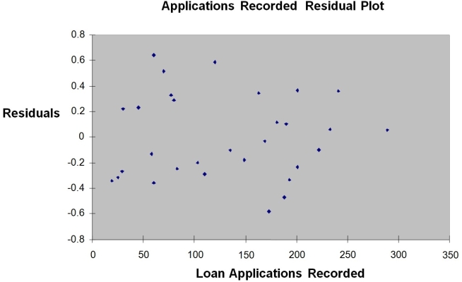
 Note: 4.3946E-15 is 4.3946 × 10⁻¹⁵.
-Referring to Instruction 12.18,the error sum of squares (SSE)of the above regression is
Note: 4.3946E-15 is 4.3946 × 10⁻¹⁵.
-Referring to Instruction 12.18,the error sum of squares (SSE)of the above regression is
(Multiple Choice)
4.9/5 (30)
The least squares method minimises which of the following?
(Multiple Choice)
4.8/5 (35)
Instruction 12.38
The director of cooperative education at a university wants to examine the effect of cooperative education job experience on marketability in the workplace. She takes a random sample of four students. For these four, she finds out how many times each had a cooperative education job and how many job offers they received upon graduation. These data are presented in the table below.
Student Coop Jobs Job Oifer 1 1 4 2 2 6 3 1 3 4 0 1
-Referring to Instruction 12.38,suppose the director of cooperative education wants to obtain a 95% prediction interval for the number of job offers received by a student who has had exactly two cooperative education jobs.The t critical value she would use is __________.
(Short Answer)
4.9/5 (43)
Filters
- Essay(0)
- Multiple Choice(0)
- Short Answer(0)
- True False(0)
- Matching(0)