Exam 12: Simple Linear Regression

Instruction 12.32 It is believed that average grade (based on a four-point scale) should have a positive linear relationship with university entrance exam scores. Given below is the Microsoft Excel output from regressing average grade on university entrance exam scores using a data set of eight randomly chosen students from a large university. $\text { Regressing average grade on university entrance exam score }$ $\text { Regression statistics }$ MultipleR 0.7598 R Square 0.5774 Adjusted R Square 0.5069 Standard Error 0.2691 Observations 8 $\text { ANOVA }$ df 55 MS F Significance F Regression 1 0.5940 0.5940 8.1986 0.0286 Residual 6 0.4347 0.0724 Total 7 1.0287 Coefficients Standard Error tStat p-value Lower 95\% Upper 95\% Intercept 0.5681 0.9284 0.6119 0.5630 -1.7036 2.8398 University entrance exam score 0.1021 0.0356 2.8633 0.0286 0.0148 0.1895 -Referring to Instruction 12.32,what are the decision and conclusion on testing whether there is any linear relationship at 1% level of significance between average grade and university entrance exam scores?

Instruction 12.13 The managers of a brokerage firm are interested in finding out if the number of new customers a broker brings into the firm affects the sales generated by the broker. They sample 12 brokers and determine the number of new customers they have enrolled in the last year and their sales amounts in thousands of dollars. These data are presented in the table that follows. Broker Clients Sales 1 27 52 2 11 37 3 42 64 4 33 55 5 15 29 6 15 34 7 25 58 8 36 59 9 28 44 10 30 48 11 17 31 12 22 38 -Referring to Instruction 12.13,the coefficient of determination is ____________.

Instruction 12.5 The managing partner of an advertising agency believes that his company's sales are related to the industry sales. He uses Microsoft Excel's Data Analysis tool to analyse the last four years of quarterly data with the following results: -Referring to Instruction 12.5,the estimates of the Y-intercept and slope are ____________ and ____________,respectively.

Instruction 12.34 The management of a chain electronic store would like to develop a model for predicting the weekly sales (in thousands of dollars) for individual stores based on the number of customers who made purchases. A random sample of 12 stores yields the following results: Customers Sales (Thousands of Dollars) 907 11.20 926 11.05 713 8.21 741 9.21 780 9.42 898 10.08 510 6.73 529 7.02 460 6.12 872 9.52 650 7.53 603 7.25 -Referring to Instruction 12.34,what is the value of the t test statistic when testing whether the number of customers who make purchases affects weekly sales?

Instruction 12.34 The management of a chain electronic store would like to develop a model for predicting the weekly sales (in thousands of dollars) for individual stores based on the number of customers who made purchases. A random sample of 12 stores yields the following results: Customers Sales (Thousands of Dollars) 907 11.20 926 11.05 713 8.21 741 9.21 780 9.42 898 10.08 510 6.73 529 7.02 460 6.12 872 9.52 650 7.53 603 7.25 -Referring to Instruction 12.34,the average weekly sales will increase by an estimated $10 for each additional purchasing customer.

The strength of the linear relationship between two numerical variables may be measured by the

onfident that the mean amount of time needed to record one additional loan application is somewhere $\text { Regression statistics }$ MultipleR 0.9447 R Square 0.8924 Adjusted R Square 0.8886 Standard Error 0.3342 Observations 30 $\text { ANOVA }$ df S5 MS F Significance F Regression 1 25.9438 25.9438 232.2200 4.3946-15 Residual 28 3.1282 0.1117 Total 29 29.072 Coefficients Standard Error tStat p-value Lower 95\% Upper 95\% Intercept 0.4024 0.1236 3.2559 0.0030 0.1492 0.6555 Applications Recorded 0.0126 0.0008 15.2388 4.3946- 15 0.0109 0.0143 $\text { Note: } 4.3946 \mathrm { E } - 15 \text { is } 4.3946 \times 10 ^ { - 15 } \text {. }$ -Referring to Instruction 12.36,the degrees of freedom for the t test on whether the number of loan applications recorded affects the amount of time are

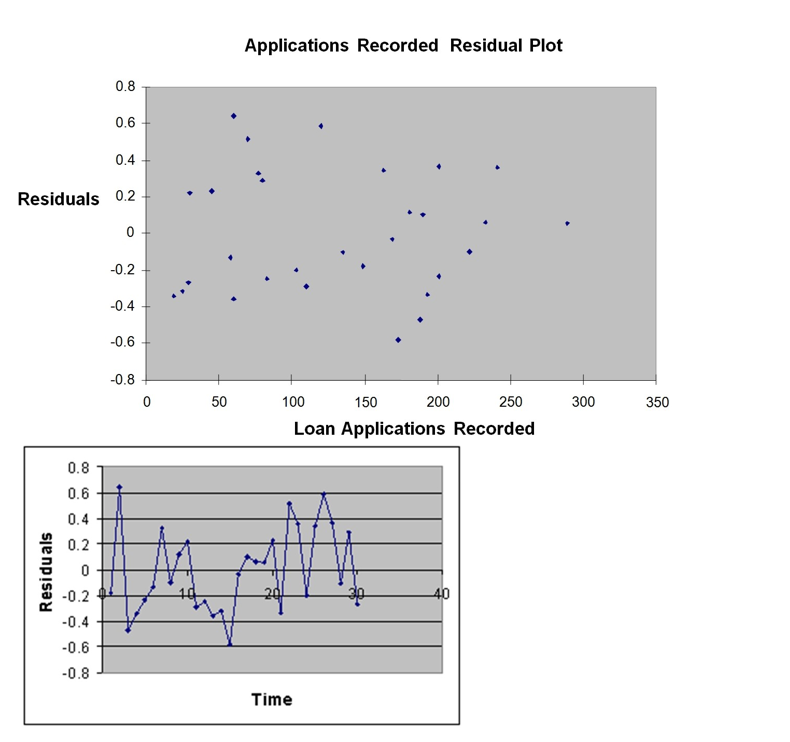
Instruction 12.22 The manager of the purchasing department of a large savings and loan organization would like to develop a model to predict the amount of time (measured in hours) it takes to record a loan application. Data are collected from a sample of 30 days, and the number of applications recorded and completion time in hours is recorded. Below is the regression output: $\text { Regression statistics }$ MultipleR 0.9447 R Square 0.8924 Adjusted R Square 0.8886 Standard Error 0.3342 Observations 30 $\text { ANOVA }$ df S5 MS F Significance F Regression 1 25.9438 25.9438 232.2200 4.3946-15 Residual 28 3.1282 0.1117 Total 29 29.072 Coefficients Standard Error tStat p-value Lower 95\% Upper 95\% Intercept 0.4024 0.1236 3.2559 0.0030 0.1492 0.6555 Applications Recorded 0.0126 0.0008 15.2388 4.3946- 15 0.0109 0.0143 Note: 4.3946E-15 is 4.3946 × 10^-15. 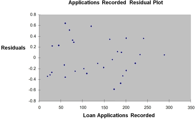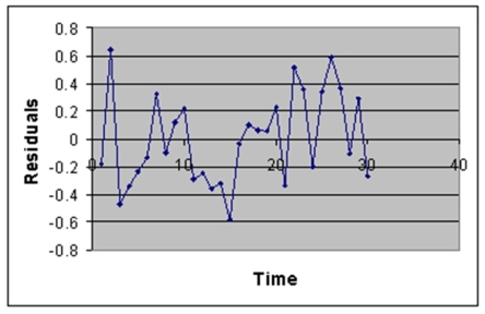-Referring to Instruction 12.22,the model appears to be adequate based on the residual analyses.

Instruction 12.5 The managing partner of an advertising agency believes that his company's sales are related to the industry sales. He uses Microsoft Excel's Data Analysis tool to analyse the last four years of quarterly data with the following results: -Referring to Instruction 12.5,the prediction for a quarter in which X = 120 is Y = ____________.

If the residuals in a regression analysis of time ordered data are not correlated,the value of the Durbin-Watson D statistic should be near____________.

The Y-intercept (b₀)represents the

Instruction 12.23 The managing partner of an advertising agency believes that his company's sales are related to the industry sales. He uses Microsoft Excel's Data Analysis tool to analyse the last four years of quarterly data with the following results: $\text { Regression statistics }$ Multiple R 0.802 R Square 0.643 Adjusted R Square 0.618 Standard Error SYX 0.9224 Observations 16 $\text { ANOVA }$ df SS MS F Sig.F Regression 1 21.497 21.497 25.27 0.000 Error 14 11.912 0.851 Total 15 33.409 Predictor Coef StdError t Stat p-value Intercept 3.962 1.440 2.75 0.016 Industry 0.040451 0.008048 5.03 0.000 Durbin-Watson 1.59 Statistic -Referring to Instruction 12.23,the partner wants to test for autocorrelation using the Durbin-Watson statistic.Using a level of significance of 0.05,the critical values of the test are d_L = ____________,and d_U =____________.

Instruction 12.38 The director of cooperative education at a university wants to examine the effect of cooperative education job experience on marketability in the workplace. She takes a random sample of four students. For these four, she finds out how many times each had a cooperative education job and how many job offers they received upon graduation. These data are presented in the table below. Student Coop Jobs Job Oifer 1 1 4 2 2 6 3 1 3 4 0 1 -Referring to Instruction 12.38,suppose the director of cooperative education wants to obtain a 95% confidence interval estimate for the mean number of job offers received by students who have had exactly one cooperative education job.The confidence interval is from __________ to __________.

Instruction 12.29 The managers of a brokerage firm are interested in finding out if the number of new customers a broker brings into the firm affects the sales generated by the broker. They sample 12 brokers and determine the number of new customers they have enrolled in the last year and their sales amounts in thousands of dollars. These data are presented in the table that follows. Broker Clients Sales 1 27 52 2 11 37 3 42 64 4 33 55 5 15 29 6 15 34 7 25 58 8 36 59 9 28 44 10 30 48 11 17 31 12 22 38 -Referring to Instruction 12.29,the managers of the brokerage firm wanted to test the hypothesis that the number of new customers brought in had a positive impact on the amount of sales generated.The p-value of the test is ____________.

The regression sum of squares (SSR)can never be greater than the total sum of squares (SST).

Instruction 12.9 The management of a chain electronic store would like to develop a model for predicting the weekly sales (in thousands of dollars) for individual stores based on the number of customers who made purchases. A random sample of 12 stores yields the following results: Customers Sales (Thousands of Dollars) 907 11.20 926 11.05 713 8.21 741 9.21 780 9.42 898 10.08 510 6.73 529 7.02 460 6.12 872 9.52 650 7.53 603 7.25 -Referring to Instruction 12.9,what are the values of the estimated intercept and slope?

Instruction 12.27 The director of cooperative education at a university wants to examine the effect of cooperative education job experience on marketability in the workplace. She takes a random sample of four students. For these four, she finds out how many times each had a cooperative education job and how many job offers they received upon graduation. These data are presented in the table below. Student Coop jobs job Offer 1 1 4 2 2 6 3 1 3 4 0 1 -Referring to Instruction 12.27,the director of cooperative education wanted to test the hypothesis that the true slope was equal to 0.For a test with a level of significance of 0.05,the null hypothesis should be rejected if the value of the test statistic is____________.

Instruction 12.34 The management of a chain electronic store would like to develop a model for predicting the weekly sales (in thousands of dollars) for individual stores based on the number of customers who made purchases. A random sample of 12 stores yields the following results: Customers Sales (Thousands of Dollars) 907 11.20 926 11.05 713 8.21 741 9.21 780 9.42 898 10.08 510 6.73 529 7.02 460 6.12 872 9.52 650 7.53 603 7.25 -Referring to Instruction 12.34,what is the p-value of the t test statistic when testing whether the number of customers who make purchases affects weekly sales?

Instruction 12.31 An investment specialist claims that if one holds a portfolio that moves in opposite direction to the market index like the All Ordinaries Index, then it is possible to reduce the variability of the portfolio's return. In other words, one can create a portfolio with positive returns but less exposure to risk. A sample of 26 years of the All Ordinaries index and a portfolio consisting of stocks of private prisons, which are believed to be negatively related to the All Ordinaries index, is collected. A regression analysis was performed by regressing the returns of the prison stocks portfolio (Y) on the returns of All Ordinaries index (X) to prove that the prison stocks portfolio is negatively related to the All Ordinaries index at a 5% level of significance. The results are given in the following Microsoft Excel output. Coefflelents Standard Error tStat p -vahse Intercept 4.866004258 0.35743609 13.61363441 8.7932-13 S\&P -0.502513506 0.071597152 -7.01862425 2.94942-07 -Referring to Instruction 12.31,to test whether the prison stocks portfolio is negatively related to the All Ordinaries index,the appropriate null and alternative hypotheses are,________- respectively,

Instruction 12.14 The managing partner of an advertising agency believes that his company's sales are related to the industry sales. He uses Microsoft Excel's Data Analysis tool to analyse the last four years of quarterly data with the following results: $\text { Regression statistics }$ Multiple R 0.802 R Square 0.643 Adjusted R Square 0.618 Standard Error SYX 0.9224 Observations 16 $\text { ANOVA }$ df SS MS F Sig.F Regression 1 21.497 21.497 25.27 0.000 Error 14 11.912 0.851 Total 15 33.409 Predictor Coef StdError t Stat p-value Intercept 3.962 1.440 2.75 0.016 Industry 0.040451 0.008048 5.03 0.000 Durbin-Watson 1.59 Statistic -Referring to Instruction 12.14,the standard error of the estimated slope coefficient is ____________.