Question 1

The residual represents the discrepancy between the observed dependent variable and itsvalue.

Accepted Answer

predicted

Question 2

SCENARIO 12-4
The managers of a brokerage firm are interested in finding out if the number of new clients a broker brings into the firm affects the sales generated by the broker.They sample 12 brokers and determine the number of new clients they have enrolled in the last year and their sales amounts in thousands of dollars.These data are presented in the table that follows. $\begin{array}{lll}
\text { Broker } & \text {Clients} & \text {Sales }\
1 & 27 & 52 \
2 & 11 & 37 \
3 & 42 & 64 \
4 & 33 & 55 \
5 & 15 & 29 \
6 & 15 & 34 \
7 & 25 & 58 \
8 & 36 & 59 \
9 & 28 & 44 \
10 & 30 & 48 \
11 & 17 & 31 \
12 & 22 & 38
\end{array}$
-Referring to Scenario 12-4, % of the total variation in sales generated can be explained by the number of new clients brought in.

Accepted Answer

The answer of SCENARIO 12-4
The managers of a brokerage firm...

Question 3

SCENARIO 12-11
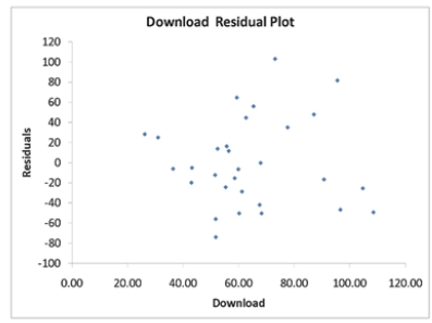
A computer software developer would like to use the number of downloads (in thousands) for the trial version of his new shareware to predict the amount of revenue (in thousands of dollars) he can make on the full version of the new shareware.Following is the output from a simple linear regression
along with the residual plot and normal probability plot obtained from a data set of 30 different sharewares that he has developed:
   $\begin{array}{lr}
{\text { Regression Statistics }} \
\hline \text { Multiple R } & 0.8691 \
\hline \text { R Square } & 0.7554 \
\hline \text { Adjusted R Square } & 0.7467 \
\hline \text { Standard Error } & 44.4765 \
\hline \text { Observations } & 30.0000 \
\hline
\end{array}$

$\text { ANOVA }$ 
$\begin{array}{|l|r|r|r|r|r|}
\hline &\text { df } & \text { SS } & \text { MS } & F & \text { Significance } F \ 
\hline \text { Regression } & 1 & 171062.9193 & 171062.9193 & 86.4759 & 0.0000 \
\hline \text { Residual } & 28 & 55388.4309 & 1978.1582 & & \
\hline \text { Total } & 29 & 226451.3503 & & \
\hline
\end{array}$

Simple Linear Regression 12-41  
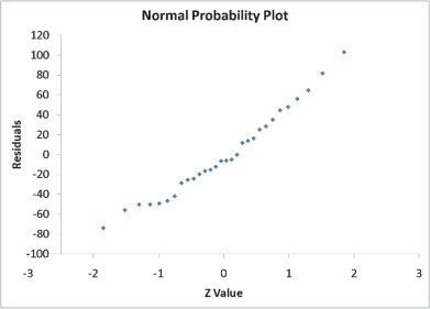-Referring to Scenario 12-11, what do the lower and upper limits of the 95% confidence interval estimate for population slope?

Accepted Answer

2.9082 and

Question 4

SCENARIO 12-12
The manager of the purchasing department of a large saving and loan organization would like to develop a model to predict the amount of time (measured in hours) it takes to record a loan
application.Data are collected from a sample of 30 days, and the number of applications recorded and completion time in hours is recorded.Below is the regression output: \[\begin{array}{l}
\begin{array} { l r } 
\hline  { \text { Regression Statistics } } \
\hline \text { Multiple R } & 0.9447 \
\text { R Square } & 0.8924 \
\text { Adjusted R } & 0.8886 \
\text { Square } & \
\text { Standard } & 0.3342 \
\text { Error } & \
\text { Observations } & 30 \
\hline
\end{array}\
\text { ANOVA }\
\begin{array} { l r r r r r } 
\hline & { \text { df } } & { \text { SS } } & { \text { MS } } & \text { F } & \text { Significance } F \
\hline \text { Regression } & 1 & 25.9438 & 25.9438 & 232.2200 & 4.3946 \mathrm { E } - 15 \
\text { Residual } & 28 & 3.1282 & 0.1117 & & \
\text { Total } & 29 & 29.072 & & & \
\hline
\end{array}\
\begin{array} { l r r r r r r } 
\hline & \text { Coefficients } & \text { Standard Error } & t \text { Stat } & \text { P-value } & \text { Lower 95\% } & \text { Upper 95\% } \
\hline \text { Intercept } & 0.4024 & 0.1236 & 3.2559 & 0.0030 & 0.1492 & 0.6555 \
\text { Applications } & 0.0126 & 0.0008 & 15.2388 & 0.0000 & 0.0109 & 0.0143 \
\text { Recorded } & & & & & & \
\hline
\end{array}
\end{array}\] 12-46 Simple Linear Regression 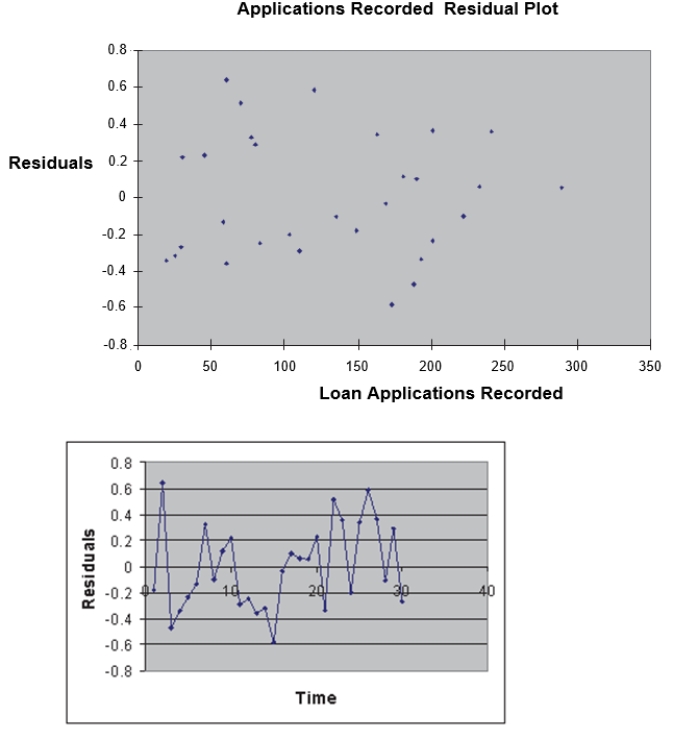  Simple Linear Regression 12-47
-Referring to Scenario 12-12, there is a 95% probability that the mean amount of time needed to record one additional loan application is somewhere between 0.0109 and 0.0143 hours.

Accepted Answer

A) True 
 B)False

Question 5

SCENARIO 12-3
The director of cooperative education at a state college wants to examine the effect of cooperative education job experience on marketability in the work place.She takes a random sample of 4 students.For these 4, she finds out how many times each had a cooperative education job and how many job offers they received upon graduation.These data are presented in the table below. $\begin{array} {ccc}\text { Student } & \text { Coop Jobs  } & \text {Job Offer }\ 1 & 1 & 4 \ 2 & 2 & 6 \ 3 & 1 & 3 \ 4 & 0 & 1 \end{array}$
-Referring to Scenario 12-3, the least squares estimate of the Y-intercept is _.

Accepted Answer

The answer of SCENARIO 12-3
The director of cooperative education at...

Question 6

SCENARIO 12-3
The director of cooperative education at a state college wants to examine the effect of cooperative education job experience on marketability in the work place.She takes a random sample of 4 students.For these 4, she finds out how many times each had a cooperative education job and how many job offers they received upon graduation.These data are presented in the table below. $\begin{array} {ccc}\text { Student } & \text { Coop Jobs  } & \text {Job Offer }\ 1 & 1 & 4 \ 2 & 2 & 6 \ 3 & 1 & 3 \ 4 & 0 & 1 \end{array}$
-Referring to Scenario 12-3, the director of cooperative education wanted to test the hypothesisthat the population slope was equal to 0.The denominator of the test statistic is s $b$ 1.The value ofs in this sample is _. $b$ 1

Accepted Answer

The answer of SCENARIO 12-3
The director of cooperative education at...

Question 7

SCENARIO 12-7
An investment specialist claims that if one holds a portfolio that moves in the opposite direction to the market index like the S&P 500, then it is possible to reduce the variability of the portfolio's return.In other words, one can create a portfolio with positive returns but less exposure to risk.
A sample of 26 years of S&P 500 index and a portfolio consisting of stocks of private prisons, which are believed to be negatively related to the S&P 500 index, is collected.A regression analysis was performed by regressing the returns of the prison stocks portfolio (Y) on the returns of S&P 500 index (X) to prove that the prison stocks portfolio is negatively related to the S&P 500 index at a 5% level
of significance.The results are given in the following EXCEL output. $$\begin{array} { l r r r r } 
\hline & \text { Coefficients } &  { \text { StandardError } } & { \text { T Stat } } & { P \text {-value } } \
\hline \text { Intercept } & 4.8660 & 0.3574 & 13.6136 & 0.0000 \
\text { S\&P } & - 0.5025 & 0.0716 & - 7.0186 & 0.0000 \
\hline
\end{array}$$
-Referring to Scenario 12-7, which of the following will be a correct conclusion?

Accepted Answer

A) You cannot reject the null hypothesis and, therefore, conclude that there is sufficient evidence to show that the prisons stock portfolio and S&P 500 index are negatively related. 
B) You can reject the null hypothesis and, therefore, conclude that there is sufficient evidence to show that the prisons stock portfolio and S&P 500 index are negatively related. 
C) You cannot reject the null hypothesis and, therefore, conclude that there is insufficient evidence to show that the prisons stock portfolio and S&P 500 index are negatively related. 
D) You can reject the null hypothesis and conclude that there is insufficient evidence to show that the prisons stock portfolio and S&P 500 index are negatively related. 
A) You cannot reject the null hypothesis and, therefore, conclude that there is sufficient evidence to show that the prisons stock portfolio and S&P 500 index are negatively related. 
B) You can reject the null hypothesis and, therefore, conclude that there is sufficient evidence to show that the prisons stock portfolio and S&P 500 index are negatively related. 
C) You cannot reject the null hypothesis and, therefore, conclude that there is insufficient evidence to show that the prisons stock portfolio and S&P 500 index are negatively related. 
D) You can reject the null hypothesis and conclude that there is insufficient evidence to show that the prisons stock portfolio and S&P 500 index are negatively related.

Question 8

SCENARIO 12-10
The management of a chain electronic store would like to develop a model for predicting the weekly sales (in thousands of dollars) for individual stores based on the number of customers who made purchases.A random sample of 12 stores yields the following results: $$\begin{array} { | l | c | } 
\hline \text { Customers } & \begin{array} { l } 
\text { Sales } \
\text { (Thousands of } \
\text { Dollars) }
\end{array} \
\hline 907 & 11.20 \
\hline 926 & 11.05 \
\hline 713 & 8.21 \
\hline 741 & 9.21 \
\hline 780 & 9.42 \
\hline 898 & 10.08 \
\hline 510 & 6.73 \
\hline 529 & 7.02 \
\hline 460 & 6.12 \
\hline 872 & 9.52 \
\hline 650 & 7.53 \
\hline 603 & 7.25 \
\hline
\end{array}$$
-Referring to Scenario 12-10, it is inappropriate to compute the Durbin-Watson statistic and test for autocorrelation in this case.

Accepted Answer

A) True 
 B)False

Question 9

SCENARIO 12-11
A computer software developer would like to use the number of downloads (in thousands) for the trial version of his new shareware to predict the amount of revenue (in thousands of dollars) he can make on the full version of the new shareware.Following is the output from a simple linear regression
along with the residual plot and normal probability plot obtained from a data set of 30 different sharewares that he has developed:
   $\begin{array}{lr}
{\text { Regression Statistics }} \
\hline \text { Multiple R } & 0.8691 \
\hline \text { R Square } & 0.7554 \
\hline \text { Adjusted R Square } & 0.7467 \
\hline \text { Standard Error } & 44.4765 \
\hline \text { Observations } & 30.0000 \
\hline
\end{array}$

$\text { ANOVA }$ 
$\begin{array}{|l|r|r|r|r|r|}
\hline &\text { df } & \text { SS } & \text { MS } & F & \text { Significance } F \ 
\hline \text { Regression } & 1 & 171062.9193 & 171062.9193 & 86.4759 & 0.0000 \
\hline \text { Residual } & 28 & 55388.4309 & 1978.1582 & & \
\hline \text { Total } & 29 & 226451.3503 & & \
\hline
\end{array}$

Simple Linear Regression 12-41  
-Referring to Scenario 12-11, the null hypothesis that there is no linear relationship between revenue and the number of downloads should be rejected at a 5% level of significance.

Accepted Answer

A) True 
 B)False

Question 10

If the correlation coefficient (r) = 1.00, then

Accepted Answer

A) all the data points must fall exactly on a straight line with a slope that equals 1.00. 
B) all the data points must fall exactly on a straight line with a negative slope. 
C) all the data points must fall exactly on a straight line with a positive slope. 
D) all the data points must fall exactly on a horizontal straight line with a zero slope. 
A) all the data points must fall exactly on a straight line with a slope that equals 1.00. 
B) all the data points must fall exactly on a straight line with a negative slope. 
C) all the data points must fall exactly on a straight line with a positive slope. 
D) all the data points must fall exactly on a horizontal straight line with a zero slope.

Question 11

SCENARIO 12-4
The managers of a brokerage firm are interested in finding out if the number of new clients a broker brings into the firm affects the sales generated by the broker.They sample 12 brokers and determine the number of new clients they have enrolled in the last year and their sales amounts in thousands of dollars.These data are presented in the table that follows. $\begin{array}{lll}
\text { Broker } & \text {Clients} & \text {Sales }\
1 & 27 & 52 \
2 & 11 & 37 \
3 & 42 & 64 \
4 & 33 & 55 \
5 & 15 & 29 \
6 & 15 & 34 \
7 & 25 & 58 \
8 & 36 & 59 \
9 & 28 & 44 \
10 & 30 & 48 \
11 & 17 & 31 \
12 & 22 & 38
\end{array}$
-Referring to Scenario 12-4, the error or residual sum of squares (SSE) is .

Accepted Answer

The answer of SCENARIO 12-4
The managers of a brokerage firm...

Question 12

SCENARIO 12-4
The managers of a brokerage firm are interested in finding out if the number of new clients a broker brings into the firm affects the sales generated by the broker.They sample 12 brokers and determine the number of new clients they have enrolled in the last year and their sales amounts in thousands of dollars.These data are presented in the table that follows. $\begin{array}{lll}
\text { Broker } & \text {Clients} & \text {Sales }\
1 & 27 & 52 \
2 & 11 & 37 \
3 & 42 & 64 \
4 & 33 & 55 \
5 & 15 & 29 \
6 & 15 & 34 \
7 & 25 & 58 \
8 & 36 & 59 \
9 & 28 & 44 \
10 & 30 & 48 \
11 & 17 & 31 \
12 & 22 & 38
\end{array}$
-Referring to Scenario 12-4, the managers of the brokerage firm wanted to test the hypothesis that the number of new clients brought in had a positive impact on the amount of sales generated.The p-value of the test is .

Accepted Answer

< 0.005 using the Ta

Question 13

SCENARIO 12-10
The management of a chain electronic store would like to develop a model for predicting the weekly sales (in thousands of dollars) for individual stores based on the number of customers who made purchases.A random sample of 12 stores yields the following results: $$\begin{array} { | l | c | } 
\hline \text { Customers } & \begin{array} { l } 
\text { Sales } \
\text { (Thousands of } \
\text { Dollars) }
\end{array} \
\hline 907 & 11.20 \
\hline 926 & 11.05 \
\hline 713 & 8.21 \
\hline 741 & 9.21 \
\hline 780 & 9.42 \
\hline 898 & 10.08 \
\hline 510 & 6.73 \
\hline 529 & 7.02 \
\hline 460 & 6.12 \
\hline 872 & 9.52 \
\hline 650 & 7.53 \
\hline 603 & 7.25 \
\hline
\end{array}$$
-Referring to Scenario 12-10, what are the degrees of freedom of the F test statistic when testing whether the number of customers who make purchases is a good predictor for weekly sales?

Accepted Answer

1 in the n

Question 14

SCENARIO 12-10
The management of a chain electronic store would like to develop a model for predicting the weekly sales (in thousands of dollars) for individual stores based on the number of customers who made purchases.A random sample of 12 stores yields the following results: $$\begin{array} { | l | c | } 
\hline \text { Customers } & \begin{array} { l } 
\text { Sales } \
\text { (Thousands of } \
\text { Dollars) }
\end{array} \
\hline 907 & 11.20 \
\hline 926 & 11.05 \
\hline 713 & 8.21 \
\hline 741 & 9.21 \
\hline 780 & 9.42 \
\hline 898 & 10.08 \
\hline 510 & 6.73 \
\hline 529 & 7.02 \
\hline 460 & 6.12 \
\hline 872 & 9.52 \
\hline 650 & 7.53 \
\hline 603 & 7.25 \
\hline
\end{array}$$
-Referring to Scenario 12-10, the value of the F test statistic equals the square of the t test statistic when testing whether the number of customers who make purchases is a good predictor for weekly sales.

Accepted Answer

A) True 
 B)False

Question 15

When r = - 1, it indicates a perfect relationship between X and Y.

Accepted Answer

A) True 
 B)False

Question 16

SCENARIO 12-3
The director of cooperative education at a state college wants to examine the effect of cooperative education job experience on marketability in the work place.She takes a random sample of 4 students.For these 4, she finds out how many times each had a cooperative education job and how many job offers they received upon graduation.These data are presented in the table below. $\begin{array} {ccc}\text { Student } & \text { Coop Jobs  } & \text {Job Offer }\ 1 & 1 & 4 \ 2 & 2 & 6 \ 3 & 1 & 3 \ 4 & 0 & 1 \end{array}$
-Referring to Scenario 12-3, the regression sum of squares (SSR) is .

Accepted Answer

The answer of SCENARIO 12-3
The director of cooperative education at...

Question 17

14.Referring to Scenario 12-2, what is the standard error of the regression slope estimate, S ?
 $$b$$ 1
a) 0.784 b) 0.885 c) 12.650 d) 16.299
ANSWER:
c
TYPE: MC DIFFICULTY: Moderate
KEYWORDS: standard error, slope
-Referring to Scenario 12-2, to test that the regression coefficient, $\beta$1, is not equal to 0, what would be the critical values? Use $\alpha$ = 0.05.

Accepted Answer

A) $\pm$ 2.5706 
B) $\pm$ 2.7764 
C) $\pm$ 3.1634 
D) $\pm$ 3.4954 
A) $\pm$ 2.5706 
B) $\pm$ 2.7764 
C) $\pm$ 3.1634 
D) $\pm$ 3.4954

Question 18

SCENARIO 12-12
The manager of the purchasing department of a large saving and loan organization would like to develop a model to predict the amount of time (measured in hours) it takes to record a loan
application.Data are collected from a sample of 30 days, and the number of applications recorded and completion time in hours is recorded.Below is the regression output: \[\begin{array}{l}
\begin{array} { l r } 
\hline  { \text { Regression Statistics } } \
\hline \text { Multiple R } & 0.9447 \
\text { R Square } & 0.8924 \
\text { Adjusted R } & 0.8886 \
\text { Square } & \
\text { Standard } & 0.3342 \
\text { Error } & \
\text { Observations } & 30 \
\hline
\end{array}\
\text { ANOVA }\
\begin{array} { l r r r r r } 
\hline & { \text { df } } & { \text { SS } } & { \text { MS } } & \text { F } & \text { Significance } F \
\hline \text { Regression } & 1 & 25.9438 & 25.9438 & 232.2200 & 4.3946 \mathrm { E } - 15 \
\text { Residual } & 28 & 3.1282 & 0.1117 & & \
\text { Total } & 29 & 29.072 & & & \
\hline
\end{array}\
\begin{array} { l r r r r r r } 
\hline & \text { Coefficients } & \text { Standard Error } & t \text { Stat } & \text { P-value } & \text { Lower 95\% } & \text { Upper 95\% } \
\hline \text { Intercept } & 0.4024 & 0.1236 & 3.2559 & 0.0030 & 0.1492 & 0.6555 \
\text { Applications } & 0.0126 & 0.0008 & 15.2388 & 0.0000 & 0.0109 & 0.0143 \
\text { Recorded } & & & & & & \
\hline
\end{array}
\end{array}\] 12-46 Simple Linear Regression   Simple Linear Regression 12-47
-Referring to Scenario 12-12, the p-value of the measured F-test statistic to test whether the number of loan applications recorded affects the amount of time is _.

Accepted Answer

The answer of SCENARIO 12-12
The manager of the purchasing department...

Question 19

SCENARIO 12-11
A computer software developer would like to use the number of downloads (in thousands) for the trial version of his new shareware to predict the amount of revenue (in thousands of dollars) he can make on the full version of the new shareware.Following is the output from a simple linear regression
along with the residual plot and normal probability plot obtained from a data set of 30 different sharewares that he has developed:
   $\begin{array}{lr}
{\text { Regression Statistics }} \
\hline \text { Multiple R } & 0.8691 \
\hline \text { R Square } & 0.7554 \
\hline \text { Adjusted R Square } & 0.7467 \
\hline \text { Standard Error } & 44.4765 \
\hline \text { Observations } & 30.0000 \
\hline
\end{array}$

$\text { ANOVA }$ 
$\begin{array}{|l|r|r|r|r|r|}
\hline &\text { df } & \text { SS } & \text { MS } & F & \text { Significance } F \ 
\hline \text { Regression } & 1 & 171062.9193 & 171062.9193 & 86.4759 & 0.0000 \
\hline \text { Residual } & 28 & 55388.4309 & 1978.1582 & & \
\hline \text { Total } & 29 & 226451.3503 & & \
\hline
\end{array}$

Simple Linear Regression 12-41  
-Referring to Scenario 12-11, what is the p-value for testing whether there is a linear relationship between revenue and the number of downloads at a 5% level of significance?

Accepted Answer

virtually

Question 20

SCENARIO 12-11
A computer software developer would like to use the number of downloads (in thousands) for the trial version of his new shareware to predict the amount of revenue (in thousands of dollars) he can make on the full version of the new shareware.Following is the output from a simple linear regression
along with the residual plot and normal probability plot obtained from a data set of 30 different sharewares that he has developed:
   $\begin{array}{lr}
{\text { Regression Statistics }} \
\hline \text { Multiple R } & 0.8691 \
\hline \text { R Square } & 0.7554 \
\hline \text { Adjusted R Square } & 0.7467 \
\hline \text { Standard Error } & 44.4765 \
\hline \text { Observations } & 30.0000 \
\hline
\end{array}$

$\text { ANOVA }$ 
$\begin{array}{|l|r|r|r|r|r|}
\hline &\text { df } & \text { SS } & \text { MS } & F & \text { Significance } F \ 
\hline \text { Regression } & 1 & 171062.9193 & 171062.9193 & 86.4759 & 0.0000 \
\hline \text { Residual } & 28 & 55388.4309 & 1978.1582 & & \
\hline \text { Total } & 29 & 226451.3503 & & \
\hline
\end{array}$

Simple Linear Regression 12-41  
-Referring to Scenario 12-11, what do the lower and upper limits of the 95% confidence interval estimate for the mean change in revenue as a result of a one thousand increase in the number of downloads?

Accepted Answer

2.9082 and

The residual represents the discrepancy between the observed dependent variable and itsvalue.

If the correlation coefficient (r) = 1.00, then

When r = - 1, it indicates a perfect relationship between X and Y.

Defining and Collecting Data

Organizing and Visualizing Variables

Numerical Descriptive Measures

Basic Probability

Discrete Probability Distributions

The Normal Distribution

Sampling Distributions

Confidence Interval Estimation

Fundamentals of Hypothesis Testing: One-Sample Tests

Two-Sample Tests

Chi-Square Tests

Multiple Regression

Business Analytics

Filters

Exam 12: Simple Linear Regression

The residual represents the discrepancy between the observed dependent variable and itsvalue.

If the correlation coefficient (r) = 1.00, then

When r = - 1, it indicates a perfect relationship between X and Y.

Defining and Collecting Data

Organizing and Visualizing Variables

Numerical Descriptive Measures

Basic Probability

Discrete Probability Distributions

The Normal Distribution

Sampling Distributions

Confidence Interval Estimation

Fundamentals of Hypothesis Testing: One-Sample Tests

Two-Sample Tests

Chi-Square Tests

Multiple Regression

Business Analytics

Filters