Exam 11: Correlation and Regression

A test was made of $H _ { 0 } : \mu _ { 1 } = \mu _ { 2 } \text { versus } H _ { 1 } : \mu _ { 1 } < \mu _ { 2 }$ The sample means $\bar { x } _ { 1 } = 7$ and $\bar { x } _ { 2 } = 13$ the sample standard deviations were $s _ { 1 } = 7 \text { and } s _ { 2 } = 5$ and the sample sizes were $n _ { 1 } = 18 \text { and } n _ { 2 } = 16$ Compute the value of the test statistic.

The bowling scores of a professional bowler during a two-day tournament are shown below 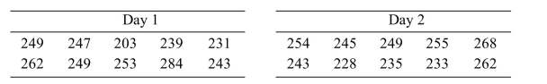Can you conclude that the variability of the scores is greater on the second day than on thi first day? Use the $\alpha = 0.01$ level of significance.

The football coach at State University wishes to determine if there is a decrease in offensive production between the first half and the second half of his team's recent games. The table below shows the first-half and second-half offensive production (measured in total yards gained per half) for the past six games. Game 1 2 3 4 5 6 First half yards 142 143 85 84 138 71 Second half yards 134 116 66 84 122 65 Compute the test statistic.

An automobile manufacturer wishes to test that claim that synthetic motor oil can improve gas mileage (in miles per gallon, or mpg). The table below shows the gas mileages, in mpg, of six cars that used synthetic motor oil. The table also shows the gas mileages in mpg of six cars that were using conventional motor oil (the controls). Synthetic: 27 27 26 27 27 29 Control: 25 25 25 26 27 25 Can you conclude that the mean gas mileage for cars using synthetic motor oil is more than the mean for the controls? Use the $\alpha = 0.05$ level of significance.

In an agricultural experiment, the effects of two fertilizers on the production of oranges were measured. Fourteen randomly selected plots of land were treated with fertilizer A, and 10 randomly selected plots were treated with fertilizer B. The The number of pounds of harvested fruit was measured from each plot. Following are the results. Fertilizer A 448 478 482 442 455 480 457 506 470 444 466 427 461 431 Fertilizer B 436 478 453 489 400 444 495 438 481 501 Assume that the populations are approximately normal. Can you conclude that there is a difference in the mean yields for the two types of fertilizer? Use the $\alpha = 0.01$ level of significance.

In a test for the difference between two proportions, the sample sizes were $n _ { 1 } = 88$ and $n _ { 2 } = 84$ and the numbers of events were $x _ { 1 } = 34 \text { and } x _ { 2 } = 39$ A test is made of the hypothesis $H _ { 0 } : p _ { 1 } = p _ { 2 } \text { versus } H _ { 1 } : p _ { 1 } \neq p _ { 2 }$ Can you reject $H _ { 0 }$ rejected at the $\alpha = 0.05$ level?

A amateur golfer wishes to determine if there is a difference between the drive distances of her two favorite drivers. (A driver is a specialized club for driving the golf ball down range. She hits fourteen balls with driver A and 10 balls with driver B. The The drive distances (in yards) for the trials are show below $\text { Driver A }$ 265 278 299 314 243 248 275 276 265 266 277 248 276 282 Driver B 233 220 217 239 235 245 261 194 272 233 Assume that the populations are approximately normal. Can you conclude that there is a difference in the mean drive distances for the two drivers? Use the $\alpha = 0.05$ level of significance.

A garden seed wholesaler wishes to test the claim that tomato seeds germinate faster when each individual seed is "pelletized" within a coating of corn starch. The table below shows the germination times, in days, of six pelletized seeds. The table also shows the germination times in days of six un-coated seeds (the controls). Pelletized: 9 9 9 8 7 8 Control: 9 10 11 13 9 11 Can you conclude that the mean germination time for pelletized seeds is less than the mean for the un-pelletized seeds? Use the $\alpha = 0.05$ level of significance.

The following MINITAB output display presents the results of a hypothesis test for the difference $\mu _ { 1 } - \mu _ { 2 }$ between two population means. Two-sample T for X1 vs X2 Mean StDev SE Mean A 7 112.415 23.485 8.876 B 8 122.788 23.222 8.210 Difference $= \operatorname { mu } ( \mathrm { X } 1 ) - \mathrm { mu } ( \mathrm { X } 2 )$ Estimate for difference: $- 10.373$ $95 \%$ CI for difference: $( - 34.072,13.326 )$ T-Test of difference $= 0 ($ vs not $= ) :$ T-Value $= - 0.857889$ $\mathrm { P }$ -Value $= 0.406493 \quad \mathrm { DF } = 13$ Can you reject $H _ { 0 }$ rejected at the $\alpha = 0.10$ level?

In an experiment to determine whether there is a systematic difference between the weights obtained with two different mass balances, six specimens were weighed, in grams, on each balance. The following data were obtained: 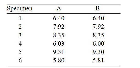Can you conclude that the mean weight differs between the two balances? i). State the null and alternative hypotheses. ii). Compute the test statistic. iii). State a conclusion using the α = 0.02 level of significance.

In a test for the difference between two proportions, the sample sizes were $n _ { 1 } = 84$ and $n _ { 2 } = 102$ and the numbers of events were $x _ { 1 } = 35 \text { and } x _ { 2 } = 64$ A test is made of the hypothesis $H _ { 0 } : p _ { 1 } = p _ { 2 } \text { versus } H _ { 1 } : p _ { 1 } \neq p _ { 2 }$ Compute the value of the test statistic.

The football coach at State University wishes to determine if there is a decrease in offensive production between the first half and the second half of his team's recent games. The table below shows the first-half and second-half offensive production (measured in total yards gained per half) for the past six games. Game 1 2 3 4 5 6 First half yards 99 127 131 106 112 144 Second half yards 89 111 129 92 103 137 State a conclusion using the $\alpha = 0.02$ level of significance.

In an experiment to determine whether there is a systematic difference between the weights obtained with two different mass balances, six specimens were weighed, in grams, on each balance. The following data were obtained: Specimen 1 14.86 14.83 2 9.44 9.41 3 11.99 11.99 4 9.27 9.26 5 6.13 6.13 6 13.78 13.76 Compute the test statistic.

A study reported that in a sample of 81 men, 25 had elevated total cholesterol levels (more than 200 milligrams per deciliter). In a sample of 99 women, 34 had elevated cholesterol levels. Can you conclude that the proportion of people with elevated cholesterol levels differs between men and women? Use the $\alpha = 0.05$ level of significance.

he following MINITAB output display presents the results of a hypothesis test on the difference between two proportions. Test and CI for Two Proportions: P1, P2 Variable Sample P P1 47 109 0.431193 P2 40 96 0.416667 Difference $= \mathrm { p } ( \mathrm { P } 1 ) = \mathrm { p } ( \mathrm { P } 2 )$ Estimate for differencę.014526 $95 \%$ CI for difference:(-0.121065, 0.150117) T-Test of difference $= 0 ($ vs not $= \not ) = 0.209977$ P-Value $= 0.833686$ Is this a left-tailed test, a right-tailed test, or a two tailed test?

The following MINITAB output display presents the results of a hypothesis test for the difference $\mu _ { 1 } - \mu _ { 2 }$ between two population means. Two-sample T for X1 vs X2 Mean StDev SE Mean A 15 71.319 24.905 6.430 B 15 50.450 24.951 6.442 Difference $= \operatorname { mu } ( \mathrm { X } 1 ) - \mathrm { mu } ( \mathrm { X } 2 )$ Estimate for difference: $20.869$ $95 \%$ CI for difference: $( 3.028,38.710 )$ T-Test of difference $= 0 ($ vs not $= ) :$ T-Value $= 2.292686$ P-Value $= 0.029586 \quad$ DF $= 28$ How many degrees of freedom are there for the test statistic?

The following display from a TI-84 Plus calculator presents the results of a hypothesis test for the difference between two means. The sample sizes are 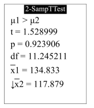$n _ { 1 } = 7 \text { and } n _ { 2 } = 15$ Can you reject $H _ { 0 }$ rejected at the $\alpha = 0.05$ level?

Following is a sample of five matched pairs. Sample 1 15 21 14 17 24 Sample 2 22 16 20 14 20 Let $\mu _ { 1 }$ and $\mu _ { 2 }$ represent the population means and let $\mu _ { \mathrm { d } } = \mu _ { 1 } - \mu _ { 2 }$ . A test will be made of the hypotheses $H _ { 0 } : \mu _ { \mathrm { d } } = 0$ versus $H _ { 1 } : \mu _ { \mathrm { d } } > 0$ . Compute the test statistic.

A test was made of $H _ { 0 } : \mu _ { 1 } = \mu _ { 2 } \text { versus } H _ { 1 } : \mu _ { 1 } < \mu _ { 2 }$ The sample means were $\bar { x } _ { 1 } = 14$ and $\bar { x } _ { 2 } = 11 \text {, }$ the sample standard deviations were $s _ { 1 } = 8 \text { and } s _ { 2 } = 4$ and the sample sizes were $n _ { 1 } = 12 \text { and } n _ { 2 } = 20$ How many degrees of freedom are there for the test statistic, using the simple method?