Exam 13: Simple Linear Regression
Exam 1: Defining and Collecting Data202 Questions
Exam 2: Organizing and Visualizing256 Questions
Exam 3: Numerical Descriptive Measures217 Questions
Exam 4: Basic Probability167 Questions
Exam 5: Discrete Probability Distributions165 Questions
Exam 6: The Normal Distribution and Other Continuous Distributions170 Questions
Exam 7: Sampling Distributions165 Questions
Exam 8: Confidence Interval Estimation219 Questions
Exam 9: Fundamentals of Hypothesis Testing: One-Sample Tests194 Questions
Exam 10: Two-Sample Tests240 Questions
Exam 11: Analysis of Variance170 Questions
Exam 12: Chi-Square and Nonparametric188 Questions
Exam 13: Simple Linear Regression243 Questions
Exam 14: Introduction to Multiple394 Questions
Exam 15: Multiple Regression146 Questions
Exam 16: Time-Series Forecasting235 Questions
Exam 17: Getting Ready to Analyze Data386 Questions
Exam 18: Statistical Applications in Quality Management159 Questions
Exam 19: Decision Making126 Questions
Exam 20: Probability and Combinatorics421 Questions
Select questions type
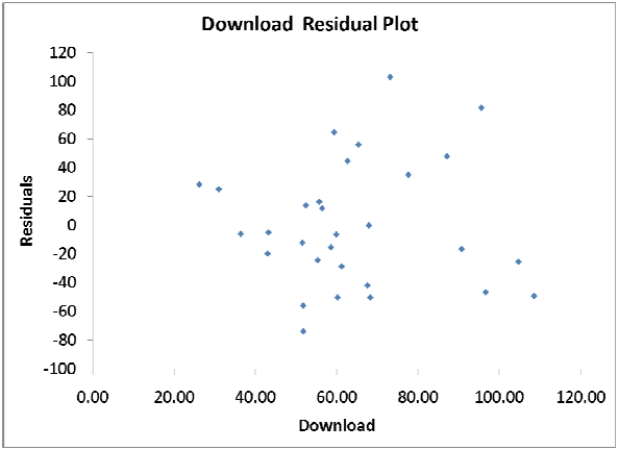
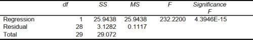
SCENARIO 13-11
A computer software developer would like to use the number of downloads (in thousands) for the trial
version of his new shareware to predict the amount of revenue (in thousands of dollars) he can make
on the full version of the new shareware. Following is the output from a simple linear regression
along with the residual plot and normal probability plot obtained from a data set of 30 different
sharewares that he has developed: 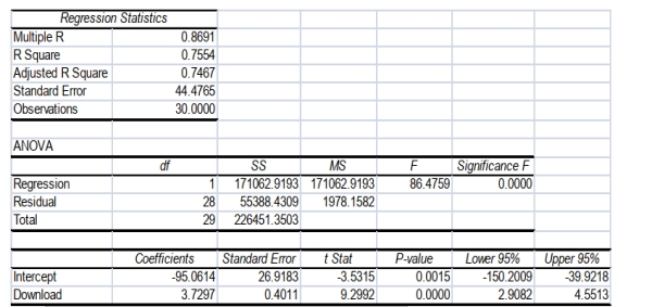
 -Referring to Scenario 13-11, what arethe lower and upper limits of the 95% confidence interval
estimate for the mean change in revenue as a result of a one thousand increase in the number of
downloads?
-Referring to Scenario 13-11, what arethe lower and upper limits of the 95% confidence interval
estimate for the mean change in revenue as a result of a one thousand increase in the number of
downloads?
(Short Answer)
4.9/5  (36)
(36)
The confidence interval for the mean of Y is always narrower than the prediction
interval for an individual response Y given the same data set, X value, and confidence level.
(True/False)
4.8/5 (39)
SCENARIO 13-9
It is believed that, the average numbers of hours spent studying per day (HOURS) during
undergraduate education should have a positive linear relationship with the starting salary (SALARY,
measured in thousands of dollars per month) after graduation. Given below is the Excel output for
predicting starting salary (Y) using number of hours spent studying per day (X) for a sample of 51
students. NOTE: Only partial output is shown. Regression Statistics Multiple R 0.8857 R Square 0.7845 Adjusted R Square 0.7801 Standard Error 1.3704 Observations 51
ANOVA
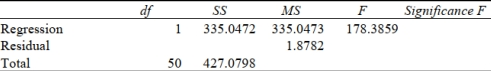
 Note: and . .
-Referring to Scenario 13-9, the error sum of squares (SSE) of the above regression is
Note: and . .
-Referring to Scenario 13-9, the error sum of squares (SSE) of the above regression is
(Multiple Choice)
4.8/5 (43)
SCENARIO 13-1
A large national bank charges local companies for using their services. A bank official reported the
results of a regression analysis designed to predict the bank's charges (Y) -- measured in dollars per
month -- for services rendered to local companies. One independent variable used to predict service
charges to a company is the company's sales revenue (X) -- measured in millions of dollars. Data for
21 companies who use the bank's services were used to fit the model:
The results of the simple linear regression are provided below.
-Referring to Scenario 13-1, interpret the p-value for testing whether exceeds 0.
(Multiple Choice)
5.0/5 (32)
EXPLANATION: The t-test statistic is KEYWORDS: t test on slope, p-value, slope
SCENARIO 13-4
The managers of a brokerage firm are interested in finding out if the number of new clients a broker
brings into the firm affects the sales generated by the broker. They sample 12 brokers and determine
the number of new clients they have enrolled in the last year and their sales amounts in thousands of
dollars. These data are presented in the table that follows. 1 27 52 2 11 37 3 42 64 4 33 55 5 15 29 6 15 34 7 25 58 8 36 59 9 28 44 10 30 48 11 17 31 12 22 38
-Referring to Scenario 13-4, the managers of the brokerage firm wanted to test the hypothesis that
the number of new clients brought in had a positive impact on the amount of sales generated. The
value of the test statistic is _______.
(Short Answer)
4.9/5 (39)
EXPLANATION: The t-test statistic is KEYWORDS: t test on slope, p-value, slope
SCENARIO 13-4
The managers of a brokerage firm are interested in finding out if the number of new clients a broker
brings into the firm affects the sales generated by the broker. They sample 12 brokers and determine
the number of new clients they have enrolled in the last year and their sales amounts in thousands of
dollars. These data are presented in the table that follows. 1 27 52 2 11 37 3 42 64 4 33 55 5 15 29 6 15 34 7 25 58 8 36 59 9 28 44 10 30 48 11 17 31 12 22 38
-Referring to Scenario 13-4, the managers of the brokerage firm wanted to test the hypothesis that
the number of new clients brought in had a positive impact on the amount of sales generated. At a
level of significance of 0.01, the null hypothesis should be _______ (rejected or not rejected).
(Short Answer)
4.8/5 (29)
SCENARIO 13-3
The director of cooperative education at a state college wants to examine the effect of cooperative
education job experience on marketability in the work place. She takes a random sample of 4
students. For these 4, she finds out how many times each had a cooperative education job and how
many job offers they received upon graduation. These data are presented in the table below. Student CoopJobs JobOffer 1 1 4 2 2 6 3 1 3 4 0 1
-Referring to Scenario 13-3, the coefficient of determination is __________.
(Short Answer)
4.8/5 (43)
SCENARIO 13-12
The manager of the purchasing department of a large saving and loan organization would like to
develop a model to predict the amount of time (measured in hours) it takes to record a loan
application. Data are collected from a sample of 30 days, and the number of applications recorded and
completion time in hours is recorded. Below is the regression output: Regression Statistics Multiple R 0.9447 R Square 0.8924 Adjusted R 0.8886 Square Standard 0.3342 Error Observations 30
 Coefficients Standard Error t Stat P-value Lower 95\% Upper 95\% Intercept 0.4024 0.1236 3.2559 0.0030 0.1492 0.6555 Applications 0.0126 0.0008 15.2388 0.0000 0.0109 0.0143
-Referring to Scenario 13-12, the p-value of the measured F-test statistic to test whether the
number of loan applications recorded affects the amount of time is _____.
Coefficients Standard Error t Stat P-value Lower 95\% Upper 95\% Intercept 0.4024 0.1236 3.2559 0.0030 0.1492 0.6555 Applications 0.0126 0.0008 15.2388 0.0000 0.0109 0.0143
-Referring to Scenario 13-12, the p-value of the measured F-test statistic to test whether the
number of loan applications recorded affects the amount of time is _____.
(Short Answer)
4.9/5 (34)
SCENARIO 13-12
The manager of the purchasing department of a large saving and loan organization would like to
develop a model to predict the amount of time (measured in hours) it takes to record a loan
application. Data are collected from a sample of 30 days, and the number of applications recorded and
completion time in hours is recorded. Below is the regression output: Regression Statistics Multiple R 0.9447 R Square 0.8924 Adjusted R 0.8886 Square Standard 0.3342 Error Observations 30
Coefficients Standard Error t Stat P-value Lower 95\% Upper 95\% Intercept 0.4024 0.1236 3.2559 0.0030 0.1492 0.6555 Applications 0.0126 0.0008 15.2388 0.0000 0.0109 0.0143
-Referring to Scenario 13-12, there is sufficient evidence that the amount of time
needed linearly depends on the number of loan applications at a 5% level of significance.
(True/False)
4.8/5 (24)
SCENARIO 13-9
It is believed that, the average numbers of hours spent studying per day (HOURS) during
undergraduate education should have a positive linear relationship with the starting salary (SALARY,
measured in thousands of dollars per month) after graduation. Given below is the Excel output for
predicting starting salary (Y) using number of hours spent studying per day (X) for a sample of 51
students. NOTE: Only partial output is shown. Regression Statistics Multiple R 0.8857 R Square 0.7845 Adjusted R Square 0.7801 Standard Error 1.3704 Observations 51
ANOVA
Note: and . .
-Referring to Scenario 13-9, to test the claim that SALARY depends positively on HOURS
against the null hypothesis that SALARY does not depend linearly on HOURS, the p-value of the
test statistic is _____.
(Short Answer)
4.9/5 (33)
SCENARIO 13-5
The managing partner of an advertising agency believes that his company's sales are related to the
industry sales. He uses Microsoft Excel to analyze the last 4 years of quarterly data with
the following results: 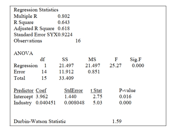 -Referring to Scenario 13-5, the estimates of the Y-intercept and slope are ________ and
________, respectively.
-Referring to Scenario 13-5, the estimates of the Y-intercept and slope are ________ and
________, respectively.
(Short Answer)
4.8/5 (34)
SCENARIO 13-13
In this era of tough economic conditions, voters increasingly ask the question: "Is the educational
achievement level of students dependent on the amount of money the state in which they reside
spends on education?" The partial computer output below is the result of using spending per student
($) as the independent variable and composite score which is the sum of the math, science and
reading scores as the dependent variable on 35 states that participated in a study. The table includes
only partial results. Regression Statistics Multiple R 0.3122 R Square 0.0975 Adjusted R 0.0701 Square Standard 26.9122 Error Observations 35
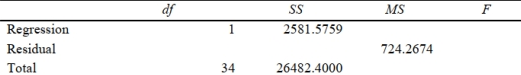
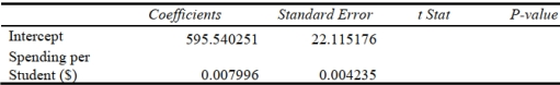 -Referring to Scenario 13-13, the value of the F test on whether spending per student affects
composite score is _________.
-Referring to Scenario 13-13, the value of the F test on whether spending per student affects
composite score is _________.
(Short Answer)
5.0/5 (31)
SCENARIO 13-3
The director of cooperative education at a state college wants to examine the effect of cooperative
education job experience on marketability in the work place. She takes a random sample of 4
students. For these 4, she finds out how many times each had a cooperative education job and how
many job offers they received upon graduation. These data are presented in the table below. Student CoopJobs JobOffer 1 1 4 2 2 6 3 1 3 4 0 1
-Referring to Scenario 13-3, the prediction for the number of job offers for a person with 2 coop
jobs is __________.
(Short Answer)
4.9/5 (33)
The least squares method minimizes which of the following?
(Multiple Choice)
4.8/5 (36)
SCENARIO 13-3
The director of cooperative education at a state college wants to examine the effect of cooperative
education job experience on marketability in the work place. She takes a random sample of 4
students. For these 4, she finds out how many times each had a cooperative education job and how
many job offers they received upon graduation. These data are presented in the table below. Student CoopJobs JobOffer 1 1 4 2 2 6 3 1 3 4 0 1
-Referring to Scenario 13-3, the director of cooperative education wanted to test the hypothesis
that the population slope was equal to 0. The denominator of the test statistic is sb1 . The value of
sb1 in this sample is ________.
(Short Answer)
4.9/5 (38)
SCENARIO 13-14-B
You are the CEO of a dairy company. You are planning to expand production by purchasing
additional cows, lands and hiring more workers. From the existing 50 farms owned by the company,
you have collected data on total milk production (in liters) and the number of milking cows. The data
are shown below and also available in the Excel file Scenario13-14-DataB.XLSX. MILK 84686 101876 103248 70508 76072 86615 87508 105195 120351 68658 85478 91902 110374 125364 159401 102883 113151 133297 140073 145434 152513 128275 138040 161276 208079 224119 231071 122114 132222 155092 177273 196399 205329 89564 94838 94920 97577 102163 103754 239585 239773 241293 249157 294388 318813 66462 100444 103846 154118 155460 COWS 21 20 22 17 16 20 21 19 21 19 22 24 26 26 27 22 27 24 27 24 29 21 25 26 33 31 33 23 27 29 27 28 32 22 26 24 26 28 26 39 44 42 41 42 47 18 21 22 27 27 You believe that the number of milking cows is the best predictor for total milk production on any
given farm.
-Referring to Scenario 13-14-B, what is the standard deviation of total milk production around
the regression line?
(Short Answer)
4.7/5 (47)
SCENARIO 13-14-A
You are the CEO of a dairy company. You are planning to expand production by purchasing
additional cows, lands and hiring more workers. From the existing 50 farms owned by the company,
you have collected data on total milk production (in liters) and the number of milking cows. The data
are shown below and also available in the Excel file Scenario13-14-DataA.XLSX. MILK 84729 101969 103314 70574 76144 86695 87600 105272 120422 68749 85541 91910 110465 125369 159470 102930 113214 133328 140086 145514 152589 128304 138093 161368 208136 224205 231090 122204 132311 155154 177268 196449 205324 89562 94840 94997 97625 102226 103832 239673 239861 241298 249196 294455 318871 66483 100459 103847 154141 155516 COWS 18 24 22 19 21 19 22 19 24 18 20 25 26 27 29 24 25 28 26 28 27 21 24 27 33 32 32 22 25 26 29 29 28 25 21 23 24 28 25 39 40 40 39 42 47 19 20 21 25 31 You believe that the number of milking cows is the best predictor for total milk production on any
given farm.
-Referring to Scenario 13-14-A, if you purchase 40 cows for the new farm, its predicted total
milk production is _________ liters.
(Short Answer)
4.9/5 (29)
SCENARIO 13-3
The director of cooperative education at a state college wants to examine the effect of cooperative
education job experience on marketability in the work place. She takes a random sample of 4
students. For these 4, she finds out how many times each had a cooperative education job and how
many job offers they received upon graduation. These data are presented in the table below. Student CoopJobs JobOffer 1 1 4 2 2 6 3 1 3 4 0 1
-Referring to Scenario 13-3, suppose the director of cooperative education wants to construct a
95% confidence-interval estimate for the mean number of job offers received by students who
have had exactly one cooperative education job. The t critical value she would use is ________.
(Short Answer)
4.8/5 (44)
Filters
- Essay(0)
- Multiple Choice(0)
- Short Answer(0)
- True False(0)
- Matching(0)