Exam 13: Simple Linear Regression
Exam 1: Defining and Collecting Data202 Questions
Exam 2: Organizing and Visualizing256 Questions
Exam 3: Numerical Descriptive Measures217 Questions
Exam 4: Basic Probability167 Questions
Exam 5: Discrete Probability Distributions165 Questions
Exam 6: The Normal Distribution and Other Continuous Distributions170 Questions
Exam 7: Sampling Distributions165 Questions
Exam 8: Confidence Interval Estimation219 Questions
Exam 9: Fundamentals of Hypothesis Testing: One-Sample Tests194 Questions
Exam 10: Two-Sample Tests240 Questions
Exam 11: Analysis of Variance170 Questions
Exam 12: Chi-Square and Nonparametric188 Questions
Exam 13: Simple Linear Regression243 Questions
Exam 14: Introduction to Multiple394 Questions
Exam 15: Multiple Regression146 Questions
Exam 16: Time-Series Forecasting235 Questions
Exam 17: Getting Ready to Analyze Data386 Questions
Exam 18: Statistical Applications in Quality Management159 Questions
Exam 19: Decision Making126 Questions
Exam 20: Probability and Combinatorics421 Questions
Select questions type
EXPLANATION: The t-test statistic is KEYWORDS: t test on slope, p-value, slope
SCENARIO 13-4
The managers of a brokerage firm are interested in finding out if the number of new clients a broker
brings into the firm affects the sales generated by the broker. They sample 12 brokers and determine
the number of new clients they have enrolled in the last year and their sales amounts in thousands of
dollars. These data are presented in the table that follows. 1 27 52 2 11 37 3 42 64 4 33 55 5 15 29 6 15 34 7 25 58 8 36 59 9 28 44 10 30 48 11 17 31 12 22 38
-Referring to Scenario 13-4, the managers of the brokerage firm wanted to test the hypothesis that
the number of new clients brought in had a positive impact on the amount of sales generated. The
p-value of the test is ________.
(Essay)
4.7/5  (42)
(42)
SCENARIO 13-11
A computer software developer would like to use the number of downloads (in thousands) for the trial
version of his new shareware to predict the amount of revenue (in thousands of dollars) he can make
on the full version of the new shareware. Following is the output from a simple linear regression
along with the residual plot and normal probability plot obtained from a data set of 30 different
sharewares that he has developed: 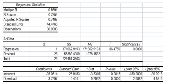
 -Referring to Scenario 13-11, which of the following is the correct alternative hypothesis for testing whether there is a linear relationship between revenue and the number of downloads? a)
b)
c)
d)
-Referring to Scenario 13-11, which of the following is the correct alternative hypothesis for testing whether there is a linear relationship between revenue and the number of downloads? a)
b)
c)
d)
(Short Answer)
4.8/5 (41)
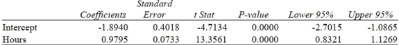
SCENARIO 13-9
It is believed that, the average numbers of hours spent studying per day (HOURS) during
undergraduate education should have a positive linear relationship with the starting salary (SALARY,
measured in thousands of dollars per month) after graduation. Given below is the Excel output for
predicting starting salary (Y) using number of hours spent studying per day (X) for a sample of 51
students. NOTE: Only partial output is shown. Regression Statistics Multiple R 0.8857 R Square 0.7845 Adjusted R Square 0.7801 Standard Error 1.3704 Observations 51
ANOVA
 Note: and . .
-Referring to Scenario 13-9, the 90% confidence interval for the average change in SALARY (in thousands of dollars) as a result of spending an extra hour per day studying is
Note: and . .
-Referring to Scenario 13-9, the 90% confidence interval for the average change in SALARY (in thousands of dollars) as a result of spending an extra hour per day studying is
(Multiple Choice)
4.8/5 (36)
SCENARIO 13-10
The management of a chain electronic store would like to develop a model for predicting the weekly
sales (in thousand of dollars) for individual stores based on the number of customers who made
purchases. A random sample of 12 stores yields the following results: Customers Sales (Thousands of Dollars) 907 11.20 926 11.05 713 8.21 741 9.21 780 9.42 898 10.08 510 6.73 529 7.02 460 6.12 872 9.52 650 7.53 603 7.25
-Referring to Scenario 13-10, generate the scatter plot.
(Essay)
4.8/5 (30)
EXPLANATION: The t-test statistic is KEYWORDS: t test on slope, p-value, slope
SCENARIO 13-4
The managers of a brokerage firm are interested in finding out if the number of new clients a broker
brings into the firm affects the sales generated by the broker. They sample 12 brokers and determine
the number of new clients they have enrolled in the last year and their sales amounts in thousands of
dollars. These data are presented in the table that follows. 1 27 52 2 11 37 3 42 64 4 33 55 5 15 29 6 15 34 7 25 58 8 36 59 9 28 44 10 30 48 11 17 31 12 22 38
-Referring to Scenario 13-4, suppose the managers of the brokerage firm want to construct both a
99% confidence interval estimate and a 99% prediction interval for X = 24. The confidence
interval estimate would be the __________ (wider or narrower) of the two intervals.
(Short Answer)
4.9/5 (42)
SCENARIO 13-9
It is believed that, the average numbers of hours spent studying per day (HOURS) during
undergraduate education should have a positive linear relationship with the starting salary (SALARY,
measured in thousands of dollars per month) after graduation. Given below is the Excel output for
predicting starting salary (Y) using number of hours spent studying per day (X) for a sample of 51
students. NOTE: Only partial output is shown. Regression Statistics Multiple R 0.8857 R Square 0.7845 Adjusted R Square 0.7801 Standard Error 1.3704 Observations 51
ANOVA
Note: and . .
-Referring to Scenario 13-9, the estimated change in mean salary (in thousands of dollars) as a result of spending an extra hour per day studying is
(Multiple Choice)
4.9/5 (39)
SCENARIO 13-10
The management of a chain electronic store would like to develop a model for predicting the weekly
sales (in thousand of dollars) for individual stores based on the number of customers who made
purchases. A random sample of 12 stores yields the following results: Customers Sales (Thousands of Dollars) 907 11.20 926 11.05 713 8.21 741 9.21 780 9.42 898 10.08 510 6.73 529 7.02 460 6.12 872 9.52 650 7.53 603 7.25
-Referring to Scenario 13-10, what is the value of the F test statistic when testing whether the
number of customers who make purchases is a good predictor for weekly sales?
(Short Answer)
4.9/5 (33)
EXPLANATION: The t-test statistic is KEYWORDS: t test on slope, p-value, slope
SCENARIO 13-4
The managers of a brokerage firm are interested in finding out if the number of new clients a broker
brings into the firm affects the sales generated by the broker. They sample 12 brokers and determine
the number of new clients they have enrolled in the last year and their sales amounts in thousands of
dollars. These data are presented in the table that follows. 1 27 52 2 11 37 3 42 64 4 33 55 5 15 29 6 15 34 7 25 58 8 36 59 9 28 44 10 30 48 11 17 31 12 22 38
-Referring to Scenario 13-4, the error or residual sum of squares (SSE) is __________.
(Short Answer)
4.8/5 (38)
SCENARIO 13-10
The management of a chain electronic store would like to develop a model for predicting the weekly
sales (in thousand of dollars) for individual stores based on the number of customers who made
purchases. A random sample of 12 stores yields the following results: Customers Sales (Thousands of Dollars) 907 11.20 926 11.05 713 8.21 741 9.21 780 9.42 898 10.08 510 6.73 529 7.02 460 6.12 872 9.52 650 7.53 603 7.25
-Referring to Scenario 13-10, the value of the t test statistic and F test statistic
should be the same when testing whether the number of customers who make purchases is a good
predictor for weekly sales.
(True/False)
4.9/5 (31)
EXPLANATION: The t-test statistic is KEYWORDS: t test on slope, p-value, slope
SCENARIO 13-4
The managers of a brokerage firm are interested in finding out if the number of new clients a broker
brings into the firm affects the sales generated by the broker. They sample 12 brokers and determine
the number of new clients they have enrolled in the last year and their sales amounts in thousands of
dollars. These data are presented in the table that follows. 1 27 52 2 11 37 3 42 64 4 33 55 5 15 29 6 15 34 7 25 58 8 36 59 9 28 44 10 30 48 11 17 31 12 22 38
-Referring to Scenario 13-4, the coefficient of determination is __________.
(Short Answer)
4.9/5 (29)
When r = - 1, it indicates a perfect relationship between X and Y.
(True/False)
4.8/5 (31)
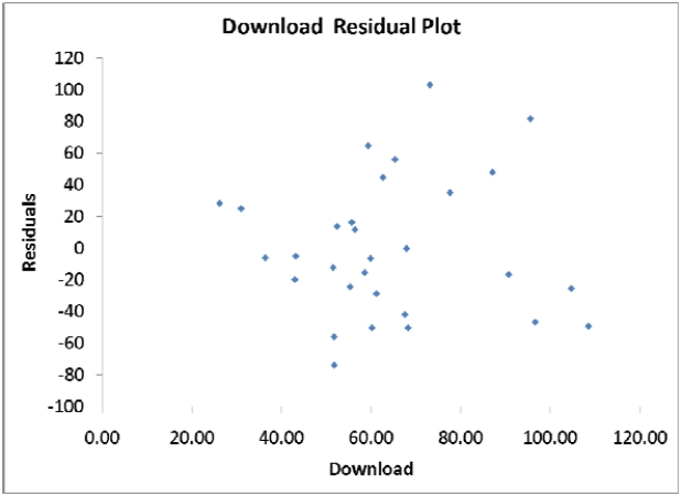
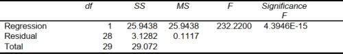
SCENARIO 13-11
A computer software developer would like to use the number of downloads (in thousands) for the trial
version of his new shareware to predict the amount of revenue (in thousands of dollars) he can make
on the full version of the new shareware. Following is the output from a simple linear regression
along with the residual plot and normal probability plot obtained from a data set of 30 different
sharewares that he has developed:
-Referring to Scenario 13-11, what arethe lower and upper limits of the 95% confidence interval
estimate for population slope?
(Short Answer)
4.8/5 (31)
EXPLANATION: The t-test statistic is KEYWORDS: t test on slope, p-value, slope
SCENARIO 13-4
The managers of a brokerage firm are interested in finding out if the number of new clients a broker
brings into the firm affects the sales generated by the broker. They sample 12 brokers and determine
the number of new clients they have enrolled in the last year and their sales amounts in thousands of
dollars. These data are presented in the table that follows. 1 27 52 2 11 37 3 42 64 4 33 55 5 15 29 6 15 34 7 25 58 8 36 59 9 28 44 10 30 48 11 17 31 12 22 38
-Referring to Scenario 13-4, the prediction for the amount of sales (in $1,000s) for a person who
brings 25 new clients into the firm is ________.
(Short Answer)
4.8/5 (33)
SCENARIO 13-13
In this era of tough economic conditions, voters increasingly ask the question: "Is the educational
achievement level of students dependent on the amount of money the state in which they reside
spends on education?" The partial computer output below is the result of using spending per student
($) as the independent variable and composite score which is the sum of the math, science and
reading scores as the dependent variable on 35 states that participated in a study. The table includes
only partial results. Regression Statistics Multiple R 0.3122 R Square 0.0975 Adjusted R 0.0701 Square Standard 26.9122 Error Observations 35
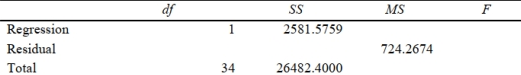
 -Referring to Scenario 13-13, the p-value of the measured t-test statistic to test whether
composite score depends linearly on spending per student is ________.
-Referring to Scenario 13-13, the p-value of the measured t-test statistic to test whether
composite score depends linearly on spending per student is ________.
(Essay)
4.8/5 (38)
Which of the following assumptions concerning the probability distribution of the random error term is stated incorrectly?
(Multiple Choice)
4.8/5 (40)
EXPLANATION: The t-test statistic is KEYWORDS: t test on slope, p-value, slope
SCENARIO 13-4
The managers of a brokerage firm are interested in finding out if the number of new clients a broker
brings into the firm affects the sales generated by the broker. They sample 12 brokers and determine
the number of new clients they have enrolled in the last year and their sales amounts in thousands of
dollars. These data are presented in the table that follows. 1 27 52 2 11 37 3 42 64 4 33 55 5 15 29 6 15 34 7 25 58 8 36 59 9 28 44 10 30 48 11 17 31 12 22 38
-Referring to Scenario 13-4, the managers of the brokerage firm wanted to test the hypothesis that
the population slope was equal to 0. At a level of significance of 0.01, the null hypothesis should
be _______ (rejected or not rejected).
(Short Answer)
4.9/5 (37)
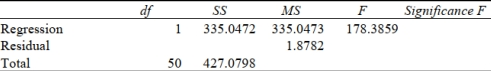
Based on the residual plot below, you will conclude that there might be a violation of which of the following assumptions. 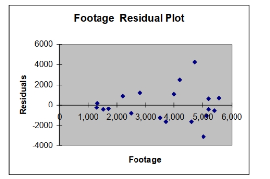
(Multiple Choice)
4.8/5 (32)
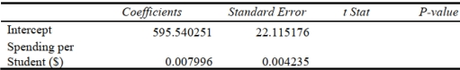
SCENARIO 13-12
The manager of the purchasing department of a large saving and loan organization would like to
develop a model to predict the amount of time (measured in hours) it takes to record a loan
application. Data are collected from a sample of 30 days, and the number of applications recorded and
completion time in hours is recorded. Below is the regression output: Regression Statistics Multiple R 0.9447 R Square 0.8924 Adjusted R 0.8886 Square Standard 0.3342 Error Observations 30
 Coefficients Standard Error t Stat P-value Lower 95\% Upper 95\% Intercept 0.4024 0.1236 3.2559 0.0030 0.1492 0.6555 Applications 0.0126 0.0008 15.2388 0.0000 0.0109 0.0143
-Referring to Scenario 13-12, what percentage of the variation in the amount of time needed can
be explained by the variation in the number of invoices processed?
Coefficients Standard Error t Stat P-value Lower 95\% Upper 95\% Intercept 0.4024 0.1236 3.2559 0.0030 0.1492 0.6555 Applications 0.0126 0.0008 15.2388 0.0000 0.0109 0.0143
-Referring to Scenario 13-12, what percentage of the variation in the amount of time needed can
be explained by the variation in the number of invoices processed?
(Short Answer)
4.9/5 (42)
SCENARIO 13-12
The manager of the purchasing department of a large saving and loan organization would like to
develop a model to predict the amount of time (measured in hours) it takes to record a loan
application. Data are collected from a sample of 30 days, and the number of applications recorded and
completion time in hours is recorded. Below is the regression output: Regression Statistics Multiple R 0.9447 R Square 0.8924 Adjusted R 0.8886 Square Standard 0.3342 Error Observations 30
Coefficients Standard Error t Stat P-value Lower 95\% Upper 95\% Intercept 0.4024 0.1236 3.2559 0.0030 0.1492 0.6555 Applications 0.0126 0.0008 15.2388 0.0000 0.0109 0.0143
-Referring to Scenario 13-12, the model appears to be adequate based on the
residual analyses.
(True/False)
4.8/5 (43)
The Regression Sum of Squares (SSR) can never be greater than the Total Sum of
Squares (SST).
(True/False)
4.8/5 (32)
Filters
- Essay(0)
- Multiple Choice(0)
- Short Answer(0)
- True False(0)
- Matching(0)