Exam 14: Introduction to Multiple Regression

In a multiple regression problem involving two independent variables,if b1 is computed to be +2.0,it means that

TABLE 14-2 A professor of industrial relations believes that an individual's wage rate at a factory (Y)depends on his performance rating (X₁)and the number of economics courses the employee successfully completed in college (X₂).The professor randomly selects 6 workers and collects the following information: 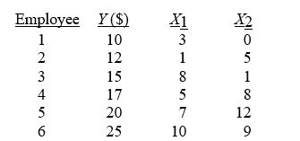-Referring to Table 14-2,an employee who took 12 economics courses scores 10 on the performance rating.What is her estimated expected wage rate?

TABLE 14-3 An economist is interested to see how consumption for an economy (in $ billions)is influenced by gross domestic product ($ billions)and aggregate price (consumer price index).The Microsoft Excel output of this regression is partially reproduced below. 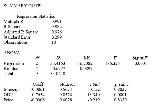-Referring to Table 14-3,what is the estimated mean consumption level for an economy with GDP equal to $2 billion and an aggregate price index of 90?

TABLE 14-17 Given below are results from the regression analysis where the dependent variable is the number of weeks a worker is unemployed due to a layoff (Unemploy)and the independent variables are the age of the worker (Age),the number of years of education received (Edu),the number of years at the previous job (Job Yr),a dummy variable for marital status (Married: 1 = married,0 = otherwise),a dummy variable for head of household (Head: 1 = yes,0 = no)and a dummy variable for management position (Manager: 1 = yes,0 = no).We shall call this Model 1.The coefficients of partial determination (R )of each of the 6 predictors are,respectively,0.2807,0.0386,0.0317,0.0141,0.0958,and 0.1201. 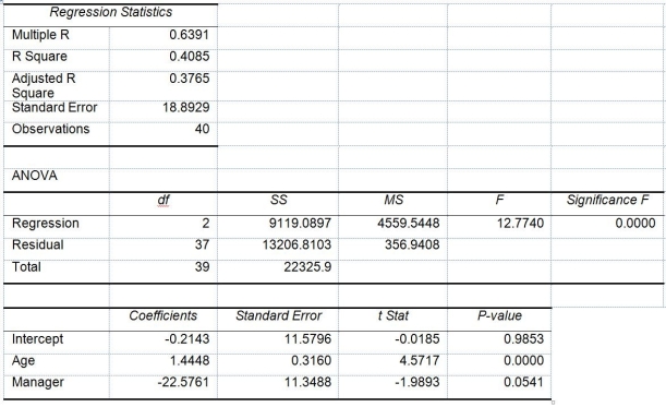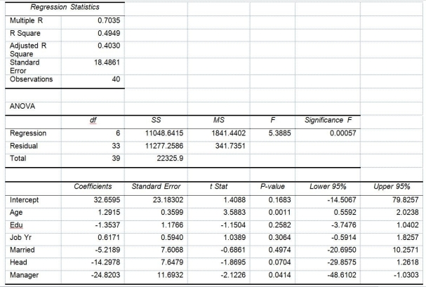Model 2 is the regression analysis where the dependent variable is Unemploy and the independent variables are Age and Manager.The results of the regression analysis are given below: -Referring to Table 14-17 Model 1,the alternative hypothesis H₁: At least one of βⱼ ≠ 0 for j = 1,2,3,4,5,6 implies that the number of weeks a worker is unemployed due to a layoff is affected by all of the explanatory variables.

TABLE 14-17 Given below are results from the regression analysis where the dependent variable is the number of weeks a worker is unemployed due to a layoff (Unemploy)and the independent variables are the age of the worker (Age),the number of years of education received (Edu),the number of years at the previous job (Job Yr),a dummy variable for marital status (Married: 1 = married,0 = otherwise),a dummy variable for head of household (Head: 1 = yes,0 = no)and a dummy variable for management position (Manager: 1 = yes,0 = no).We shall call this Model 1.The coefficients of partial determination (R )of each of the 6 predictors are,respectively,0.2807,0.0386,0.0317,0.0141,0.0958,and 0.1201. Model 2 is the regression analysis where the dependent variable is Unemploy and the independent variables are Age and Manager.The results of the regression analysis are given below: -Referring to Table 14-17 Model 1,the null hypothesis should be rejected at a 10% level of significance when testing whether being married or not makes a difference in the mean number of weeks a worker is unemployed due to a layoff while holding constant the effect of all the other independent variables.

In a multiple regression model,which of the following is correct regarding the value of the adjusted r²?

TABLE 14-3 An economist is interested to see how consumption for an economy (in $ billions)is influenced by gross domestic product ($ billions)and aggregate price (consumer price index).The Microsoft Excel output of this regression is partially reproduced below. -Referring to Table 14-3,the p-value for the regression model as a whole is

TABLE 14-2 A professor of industrial relations believes that an individual's wage rate at a factory (Y)depends on his performance rating (X₁)and the number of economics courses the employee successfully completed in college (X₂).The professor randomly selects 6 workers and collects the following information: -Referring to Table 14-2,for these data,what is the estimated coefficient for performance rating,b₁?

TABLE 14-12 As a project for his business statistics class,a student examined the factors that determined parking meter rates throughout the campus area.Data were collected for the price per hour of parking,blocks to the quadrangle,and one of the three jurisdictions: on campus,in downtown and off campus,or outside of downtown and off campus.The population regression model hypothesized is Yᵢ = α + β₁X₁ᵢ + β₂X₂ᵢ + β₃X₃ᵢ + ε where Y is the meter price X₁ is the number of blocks to the quad X₂ is a dummy variable that takes the value 1 if the meter is located in downtown and off campus and the value 0 otherwise X₃ is a dummy variable that takes the value 1 if the meter is located outside of downtown and off campus,and the value 0 otherwise The following Excel results are obtained. 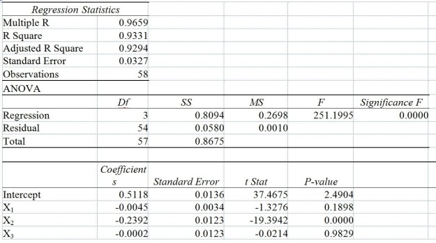-Referring to Table 14-12,predict the meter rate per hour if one parks outside of downtown and off campus 3 blocks from the quad.

TABLE 14-15 The superintendent of a school district wanted to predict the percentage of students passing a sixth-grade proficiency test.She obtained the data on percentage of students passing the proficiency test (% Passing),daily mean of the percentage of students attending class (% Attendance),mean teacher salary in dollars (Salaries),and instructional spending per pupil in dollars (Spending)of 47 schools in the state. Following is the multiple regression output with Y = % Passing as the dependent variable,X₁ = % Attendance,X₂= Salaries and X₃= Spending: 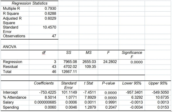-Referring to Table 14-15,you can conclude that instructional spending per pupil has no impact on the mean percentage of students passing the proficiency test,taking into account the effect of all the other independent variables,at a 5% level of significance using the 95% confidence interval estimate for β₃.

TABLE 14-15 The superintendent of a school district wanted to predict the percentage of students passing a sixth-grade proficiency test.She obtained the data on percentage of students passing the proficiency test (% Passing),daily mean of the percentage of students attending class (% Attendance),mean teacher salary in dollars (Salaries),and instructional spending per pupil in dollars (Spending)of 47 schools in the state. Following is the multiple regression output with Y = % Passing as the dependent variable,X₁ = % Attendance,X₂= Salaries and X₃= Spending: -Referring to Table 14-15,the alternative hypothesis H₁: At least one of βⱼ ≠ 0 for j = 1,2,3 implies that percentage of students passing the proficiency test is affected by all of the explanatory variables.

TABLE 14-15 The superintendent of a school district wanted to predict the percentage of students passing a sixth-grade proficiency test.She obtained the data on percentage of students passing the proficiency test (% Passing),daily mean of the percentage of students attending class (% Attendance),mean teacher salary in dollars (Salaries),and instructional spending per pupil in dollars (Spending)of 47 schools in the state. Following is the multiple regression output with Y = % Passing as the dependent variable,X₁ = % Attendance,X₂= Salaries and X₃= Spending: -Referring to Table 14-15,which of the following is the correct alternative hypothesis to test whether instructional spending per pupil has any effect on percentage of students passing the proficiency test,taking into account the effect of all the other independent variables?

TABLE 14-15 The superintendent of a school district wanted to predict the percentage of students passing a sixth-grade proficiency test.She obtained the data on percentage of students passing the proficiency test (% Passing),daily mean of the percentage of students attending class (% Attendance),mean teacher salary in dollars (Salaries),and instructional spending per pupil in dollars (Spending)of 47 schools in the state. Following is the multiple regression output with Y = % Passing as the dependent variable,X₁ = % Attendance,X₂= Salaries and X₃= Spending: -Referring to Table 14-15,the null hypothesis H₀: = β₁ = β₂ = β₃ = 0 implies that percentage of students passing the proficiency test is not affected by any of the explanatory variables.

TABLE 14-15 The superintendent of a school district wanted to predict the percentage of students passing a sixth-grade proficiency test.She obtained the data on percentage of students passing the proficiency test (% Passing),daily mean of the percentage of students attending class (% Attendance),mean teacher salary in dollars (Salaries),and instructional spending per pupil in dollars (Spending)of 47 schools in the state. Following is the multiple regression output with Y = % Passing as the dependent variable,X₁ = % Attendance,X₂= Salaries and X₃= Spending: -Referring to Table 14-15,what are the lower and upper limits of the 95% confidence interval estimate for the effect of a one dollar increase in instructional spending per pupil on the mean percentage of students passing the proficiency test?

TABLE 14-17 Given below are results from the regression analysis where the dependent variable is the number of weeks a worker is unemployed due to a layoff (Unemploy)and the independent variables are the age of the worker (Age),the number of years of education received (Edu),the number of years at the previous job (Job Yr),a dummy variable for marital status (Married: 1 = married,0 = otherwise),a dummy variable for head of household (Head: 1 = yes,0 = no)and a dummy variable for management position (Manager: 1 = yes,0 = no).We shall call this Model 1.The coefficients of partial determination (R )of each of the 6 predictors are,respectively,0.2807,0.0386,0.0317,0.0141,0.0958,and 0.1201. Model 2 is the regression analysis where the dependent variable is Unemploy and the independent variables are Age and Manager.The results of the regression analysis are given below: -Referring to Table 14-17 Model 1,which of the following is the correct alternative hypothesis to test whether age has any effect on the number of weeks a worker is unemployed due to a layoff while holding constant the effect of all the other independent variables?

When a dummy variable is included in a multiple regression model,the interpretation of the estimated slope coefficient does not make any sense anymore.

TABLE 14-17 Given below are results from the regression analysis where the dependent variable is the number of weeks a worker is unemployed due to a layoff (Unemploy)and the independent variables are the age of the worker (Age),the number of years of education received (Edu),the number of years at the previous job (Job Yr),a dummy variable for marital status (Married: 1 = married,0 = otherwise),a dummy variable for head of household (Head: 1 = yes,0 = no)and a dummy variable for management position (Manager: 1 = yes,0 = no).We shall call this Model 1.The coefficients of partial determination (R )of each of the 6 predictors are,respectively,0.2807,0.0386,0.0317,0.0141,0.0958,and 0.1201. Model 2 is the regression analysis where the dependent variable is Unemploy and the independent variables are Age and Manager.The results of the regression analysis are given below: -Referring to Table 14-17 Model 1,________ of the variation in the number of weeks a worker is unemployed due to a layoff can be explained by the number of years of education received while controlling for the other independent variables.

TABLE 14-18 A logistic regression model was estimated in order to predict the probability that a randomly chosen university or college would be a private university using information on mean total Scholastic Aptitude Test score (SAT)at the university or college,the room and board expense measured in thousands of dollars (Room/Brd),and whether the TOEFL criterion is at least 550 (Toefl550 = 1 if yes,0 otherwise.)The dependent variable,Y,is school type (Type = 1 if private and 0 otherwise). The Minitab output is given below: 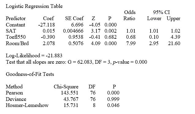-Referring to Table 14-18,what is the p-value of the test statistic when testing whether the model is a good-fitting model?

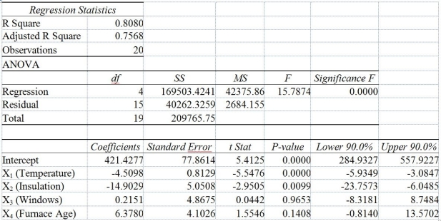
TABLE 14-6 One of the most common questions of prospective house buyers pertains to the cost of heating in dollars (Y).To provide its customers with information on that matter,a large real estate firm used the following 4 variables to predict heating costs: the daily minimum outside temperature in degrees of Fahrenheit (X₁)the amount of insulation in inches (X₂),the number of windows in the house (X₃),and the age of the furnace in years (X₄).Given below are the Excel outputs of two regression models. Model 1 Model 2 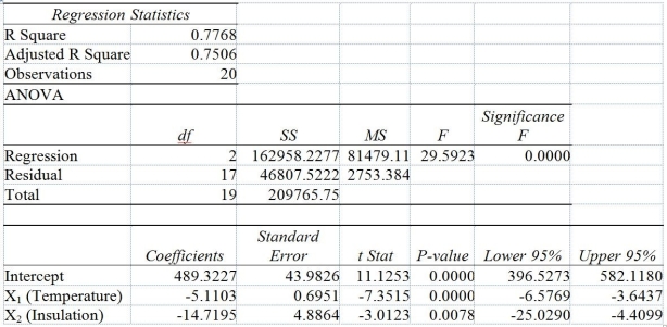-Referring to Table 14-6,what is your decision and conclusion for the test H₀: β₂ = 0 vs H₁: β₂ < 0 at the α = 0.01 level of significance using Model 1?

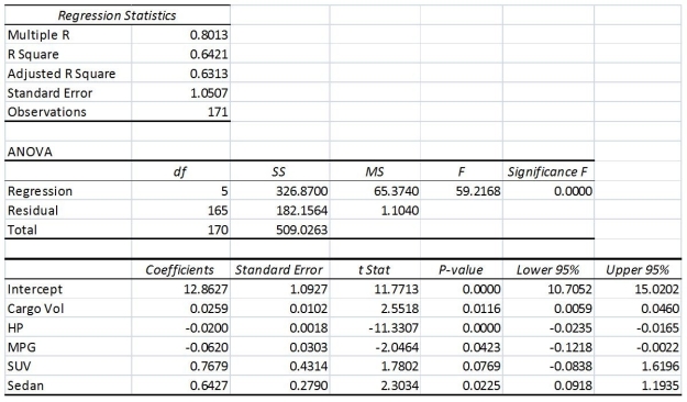
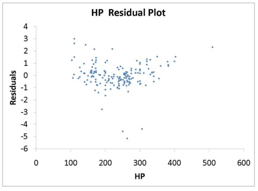
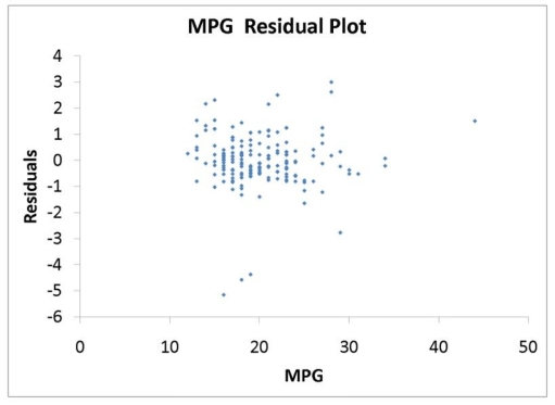
TABLE 14-16 What are the factors that determine the acceleration time (in sec.)from 0 to 60 miles per hour of a car? Data on the following variables for 171 different vehicle models were collected: Accel Time: Acceleration time in sec. Cargo Vol: Cargo volume in cu.ft. 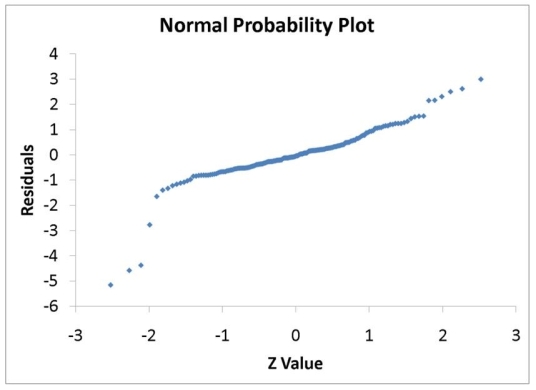HP: Horsepower MPG: Miles per gallon SUV: 1 if the vehicle model is an SUV with Coupe as the base when SUV and Sedan are both 0 Sedan: 1 if the vehicle model is a sedan with Coupe as the base when SUV and Sedan are both 0 The regression results using acceleration time as the dependent variable and the remaining variables as the independent variables are presented below. 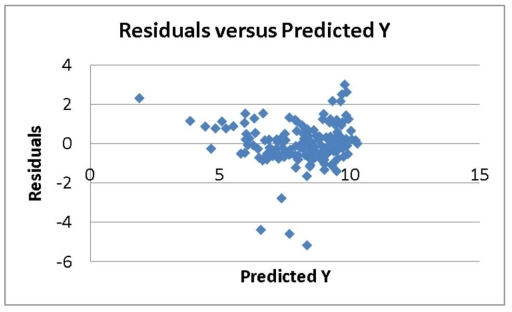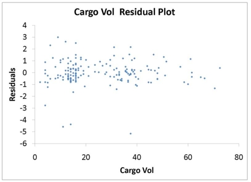The various residual plots are as shown below. The coefficients of partial determination (R )of each of the 5 predictors are,respectively,0.0380,0.4376,0.0248,0.0188,and 0.0312. The coefficient of multiple determination for the regression model using each of the 5 variables Xⱼ as the dependent variable and all other X variables as independent variables (R )are,respectively,0.7461,0.5676,0.6764,0.8582,0.6632. -Referring to 14-16,what is the value of the test statistic to determine whether SUV makes a significant contribution to the regression model in the presence of the other independent variables at a 5% level of significance?