Exam 14: Introduction to Multiple Regression

TABLE 14-8 A financial analyst wanted to examine the relationship between salary (in $1,000)and 4 variables: age (X₁ = Age),experience in the field (X₂ = Exper),number of degrees (X₃ = Degrees),and number of previous jobs in the field (X₄ = Prevjobs).He took a sample of 20 employees and obtained the following Microsoft Excel output: 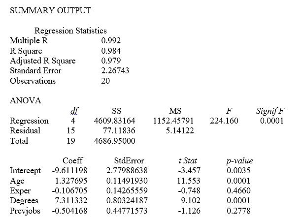-Referring to Table 14-8,the value of the adjusted coefficient of multiple determination,adj r²,is ________.

TABLE 14-3 An economist is interested to see how consumption for an economy (in $ billions)is influenced by gross domestic product ($ billions)and aggregate price (consumer price index).The Microsoft Excel output of this regression is partially reproduced below. 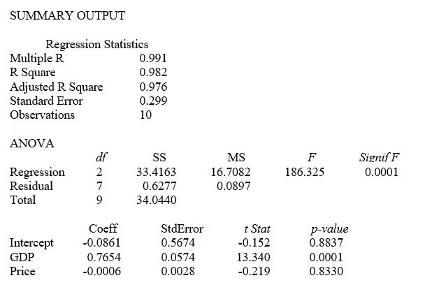-Referring to Table 14-3,to test for the significance of the coefficient on aggregate price index,the value of the relevant t-statistic is

A regression had the following results: SST = 102.55,SSE = 82.04.It can be said that 90.0% of the variation in the dependent variable is explained by the independent variables in the regression.

TABLE 14-4 A real estate builder wishes to determine how house size (House)is influenced by family income (Income),family size (Size),and education of the head of household (School).House size is measured in hundreds of square feet,income is measured in thousands of dollars,and education is in years.The builder randomly selected 50 families and ran the multiple regression.Microsoft Excel output is provided below: 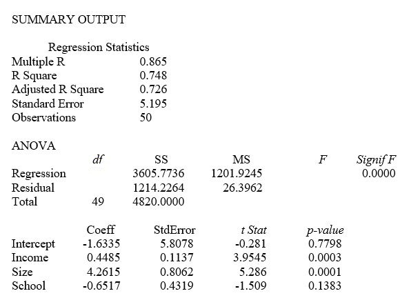-Referring to Table 14-4,which of the following values for the level of significance is the smallest for which every explanatory variable is significant individually?

TABLE 14-18 A logistic regression model was estimated in order to predict the probability that a randomly chosen university or college would be a private university using information on mean total Scholastic Aptitude Test score (SAT)at the university or college,the room and board expense measured in thousands of dollars (Room/Brd),and whether the TOEFL criterion is at least 550 (Toefl550 = 1 if yes,0 otherwise.)The dependent variable,Y,is school type (Type = 1 if private and 0 otherwise). The Minitab output is given below: 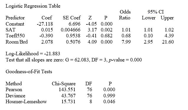-Referring to Table 14-18,there is not enough evidence to conclude that Toefl500 makes a significant contribution to the model in the presence of the other independent variables at a 0.05 level of significance.

TABLE 14-14 An automotive engineer would like to be able to predict automobile mileages.She believes that the two most important characteristics that affect mileage are horsepower and the number of cylinders (4 or 6)of a car.She believes that the appropriate model is Y = 40 - 0.05X₁ + 20X₂ - 0.1X₁X₂ where X₁ = horsepower X₂ = 1 if 4 cylinders,0 if 6 cylinders Y = mileage. -Referring to Table 14-14,the fitted model for predicting mileages for 6-cylinder cars is ________.

TABLE 14-17 Given below are results from the regression analysis where the dependent variable is the number of weeks a worker is unemployed due to a layoff (Unemploy)and the independent variables are the age of the worker (Age),the number of years of education received (Edu),the number of years at the previous job (Job Yr),a dummy variable for marital status (Married: 1 = married,0 = otherwise),a dummy variable for head of household (Head: 1 = yes,0 = no)and a dummy variable for management position (Manager: 1 = yes,0 = no).We shall call this Model 1.The coefficients of partial determination (R )of each of the 6 predictors are,respectively,0.2807,0.0386,0.0317,0.0141,0.0958,and 0.1201. 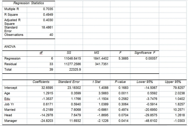Model 2 is the regression analysis where the dependent variable is Unemploy and the independent variables are Age and Manager.The results of the regression analysis are given below: -Referring to Table 14-17 and using both Model 1 and Model 2,the null hypothesis for testing whether the independent variables that are not significant individually are also not significant as a group in explaining the variation in the dependent variable should be rejected at a 5% level of significance?

When an explanatory variable is dropped from a multiple regression model,the adjusted r² can increase.

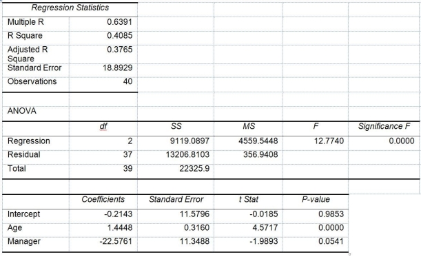
TABLE 14-15 The superintendent of a school district wanted to predict the percentage of students passing a sixth-grade proficiency test.She obtained the data on percentage of students passing the proficiency test (% Passing),daily mean of the percentage of students attending class (% Attendance),mean teacher salary in dollars (Salaries),and instructional spending per pupil in dollars (Spending)of 47 schools in the state. Following is the multiple regression output with Y = % Passing as the dependent variable,X₁ = % Attendance,X₂= Salaries and X₃= Spending: -Referring to Table 14-15,what is the p-value of the test statistic when testing whether daily average of the percentage of students attending class has any effect on percentage of students passing the proficiency test,taking into account the effect of all the other independent variables?

TABLE 14-5 A microeconomist wants to determine how corporate sales are influenced by capital and wage spending by companies.She proceeds to randomly select 26 large corporations and record information in millions of dollars.The Microsoft Excel output below shows results of this multiple regression. 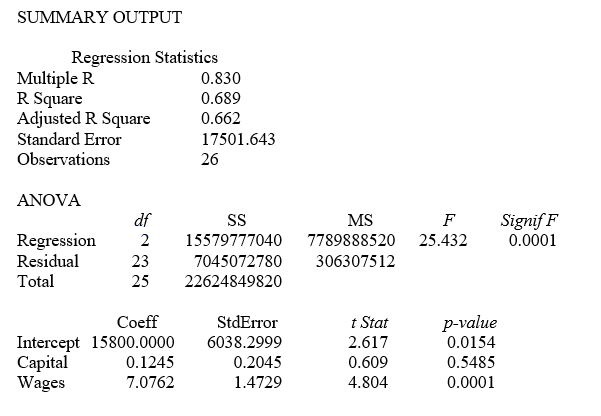-Referring to Table 14-5,what is the p-value for testing whether Wages have a negative impact on corporate sales?

TABLE 14-5 A microeconomist wants to determine how corporate sales are influenced by capital and wage spending by companies.She proceeds to randomly select 26 large corporations and record information in millions of dollars.The Microsoft Excel output below shows results of this multiple regression. -Referring to Table 14-5,what is the p-value for testing whether Capital has a positive influence on corporate sales?

TABLE 14-11 A weight-loss clinic wants to use regression analysis to build a model for weight-loss of a client (measured in pounds).Two variables thought to affect weight-loss are client's length of time on the weight-loss program and time of session.These variables are described below: Y = Weight-loss (in pounds) X₁ = Length of time in weight-loss program (in months) X₂ = 1 if morning session,0 if not X₃ = 1 if afternoon session,0 if not (Base level = evening session) Data for 12 clients on a weight-loss program at the clinic were collected and used to fit the interaction model: Y = β₀ + β₁X₁ + β₂X₂ + β₃X₃ + β₄X₁X₂ + β₅X₁X₂ + ε Partial output from Microsoft Excel follows: 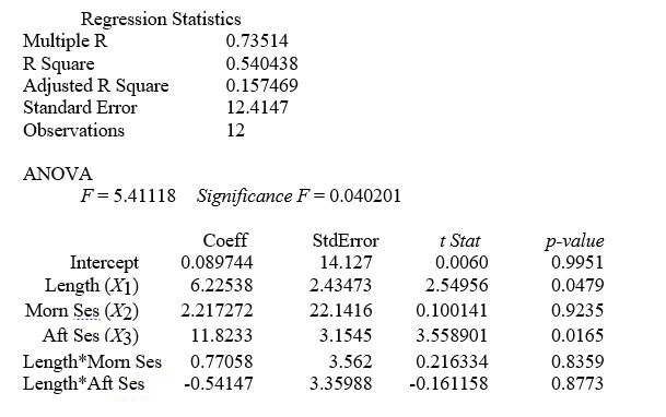-Referring to Table 14-11,in terms of the βs in the model,give the mean change in weight-loss (Y)for every 1 month increase in time in the program (X₁)when attending the morning session.

To explain personal consumption (CONS)measured in dollars,data is collected for INC: personal income in dollars CRDTLIM: $1 plus the credit limit in dollars available to the individual APR: mean annualized percentage interest rate for borrowing for the individual ADVT: per person advertising expenditure in dollars by manufacturers in the city where the individual lives A regression analysis was performed with CONS as the dependent variable and ln(CRDTLIM),ln(APR),ln(ADVT),and GENDER as the independent variables.The estimated model was Y = 2.28 - 0.29 1n(CRDTLIM)+ 5.77 1n(APR)+ 2.35 In(ADVT)+ 0.39 SEX What is the correct interpretation for the estimated coefficient for GENDER?

TABLE 14-5 A microeconomist wants to determine how corporate sales are influenced by capital and wage spending by companies.She proceeds to randomly select 26 large corporations and record information in millions of dollars.The Microsoft Excel output below shows results of this multiple regression. -Referring to Table 14-5,which of the following values for α is the smallest for which the regression model as a whole is significant?

TABLE 14-5 A microeconomist wants to determine how corporate sales are influenced by capital and wage spending by companies.She proceeds to randomly select 26 large corporations and record information in millions of dollars.The Microsoft Excel output below shows results of this multiple regression. -Referring to Table 14-5,which of the independent variables in the model are significant at the 5% level?

TABLE 14-13 An econometrician is interested in evaluating the relationship of demand for building materials to mortgage rates in Los Angeles and San Francisco.He believes that the appropriate model is Y = 10 + 5X₁ + 8X₂ where X₁ = mortgage rate in % X₂ = 1 if SF,0 if LA Y = demand in $100 per capita -Referring to Table 14-13,holding constant the effect of city,each additional increase of 1% in the mortgage rate would lead to an estimated increase of ________ in the mean demand.

TABLE 14-4 A real estate builder wishes to determine how house size (House)is influenced by family income (Income),family size (Size),and education of the head of household (School).House size is measured in hundreds of square feet,income is measured in thousands of dollars,and education is in years.The builder randomly selected 50 families and ran the multiple regression.Microsoft Excel output is provided below: -Referring to Table 14-4,one individual in the sample had an annual income of $40,000,a family size of 1,and an education of 8 years.This individual owned a home with an area of 1,000 square feet (House = 10.00).What is the residual (in hundreds of square feet)for this data point?

TABLE 14-19 The marketing manager for a nationally franchised lawn service company would like to study the characteristics that differentiate home owners who do and do not have a lawn service.A random sample of 30 home owners located in a suburban area near a large city was selected; 15 did not have a lawn service (code 0)and 15 had a lawn service (code 1).Additional information available concerning these 30 home owners includes family income (Income,in thousands of dollars),lawn size (Lawn Size,in thousands of square feet),attitude toward outdoor recreational activities (Atitude 0 = unfavorable,1 = favorable),number of teenagers in the household (Teenager),and age of the head of the household (Age). The Minitab output is given below: 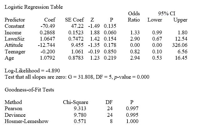-Referring to Table 14-19,there is not enough evidence to conclude that Teenager makes a significant contribution to the model in the presence of the other independent variables at a 0.05 level of significance.

TABLE 14-19 The marketing manager for a nationally franchised lawn service company would like to study the characteristics that differentiate home owners who do and do not have a lawn service.A random sample of 30 home owners located in a suburban area near a large city was selected; 15 did not have a lawn service (code 0)and 15 had a lawn service (code 1).Additional information available concerning these 30 home owners includes family income (Income,in thousands of dollars),lawn size (Lawn Size,in thousands of square feet),attitude toward outdoor recreational activities (Atitude 0 = unfavorable,1 = favorable),number of teenagers in the household (Teenager),and age of the head of the household (Age). The Minitab output is given below: -Referring to Table 14-19,what should be the decision ('reject' or 'do not reject')on the null hypothesis when testing whether Income makes a significant contribution to the model in the presence of the other independent variables at a 0.05 level of significance?

TABLE 14-15 The superintendent of a school district wanted to predict the percentage of students passing a sixth-grade proficiency test.She obtained the data on percentage of students passing the proficiency test (% Passing),daily mean of the percentage of students attending class (% Attendance),mean teacher salary in dollars (Salaries),and instructional spending per pupil in dollars (Spending)of 47 schools in the state. Following is the multiple regression output with Y = % Passing as the dependent variable,X₁ = % Attendance,X₂= Salaries and X₃= Spending: -Referring to Table 14-15,you can conclude that mean teacher salary individually has no impact on the mean percentage of students passing the proficiency test,taking into account the effect of all the other independent variables,at a 1% level of significance based solely on the 95% confidence interval estimate for β₂.