Exam 14: Introduction to Multiple Regression

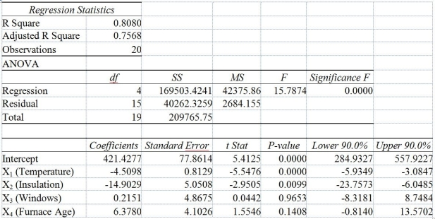
TABLE 14-6 One of the most common questions of prospective house buyers pertains to the cost of heating in dollars (Y).To provide its customers with information on that matter,a large real estate firm used the following 4 variables to predict heating costs: the daily minimum outside temperature in degrees of Fahrenheit (X₁)the amount of insulation in inches (X₂),the number of windows in the house (X₃),and the age of the furnace in years (X₄).Given below are the Excel outputs of two regression models. 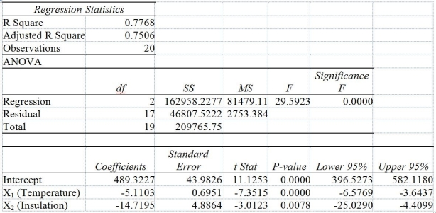Model 1 Model 2 -Referring to Table 14-6 and allowing for a 1% probability of committing a type I error,what is the decision and conclusion for the test H₀: β₁ = β₂ = β₃ = β₄ = 0 vs.H₁: At least one βⱼ ≠ 0,j = 1,2,...,4 using Model 1?

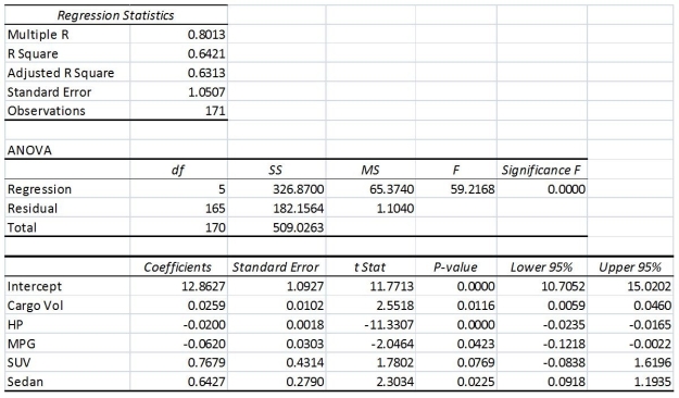
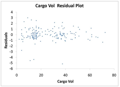
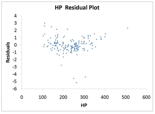
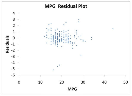
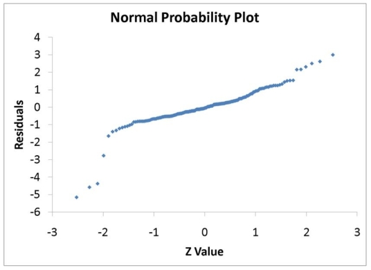
TABLE 14-16 What are the factors that determine the acceleration time (in sec.)from 0 to 60 miles per hour of a car? Data on the following variables for 171 different vehicle models were collected: Accel Time: Acceleration time in sec. Cargo Vol: Cargo volume in cu.ft. HP: Horsepower MPG: Miles per gallon SUV: 1 if the vehicle model is an SUV with Coupe as the base when SUV and Sedan are both 0 Sedan: 1 if the vehicle model is a sedan with Coupe as the base when SUV and Sedan are both 0 The regression results using acceleration time as the dependent variable and the remaining variables as the independent variables are presented below. 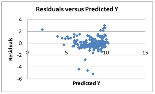The various residual plots are as shown below. The coefficients of partial determination (R )of each of the 5 predictors are,respectively,0.0380,0.4376,0.0248,0.0188,and 0.0312. The coefficient of multiple determination for the regression model using each of the 5 variables Xⱼ as the dependent variable and all other X variables as independent variables (R )are,respectively,0.7461,0.5676,0.6764,0.8582,0.6632. -Referring to 14-16,what is the correct interpretation for the estimated coefficient for SUV?

TABLE 14-16 What are the factors that determine the acceleration time (in sec.)from 0 to 60 miles per hour of a car? Data on the following variables for 171 different vehicle models were collected: Accel Time: Acceleration time in sec. Cargo Vol: Cargo volume in cu.ft. HP: Horsepower MPG: Miles per gallon SUV: 1 if the vehicle model is an SUV with Coupe as the base when SUV and Sedan are both 0 Sedan: 1 if the vehicle model is a sedan with Coupe as the base when SUV and Sedan are both 0 The regression results using acceleration time as the dependent variable and the remaining variables as the independent variables are presented below. The various residual plots are as shown below. The coefficients of partial determination (R )of each of the 5 predictors are,respectively,0.0380,0.4376,0.0248,0.0188,and 0.0312. The coefficient of multiple determination for the regression model using each of the 5 variables Xⱼ as the dependent variable and all other X variables as independent variables (R )are,respectively,0.7461,0.5676,0.6764,0.8582,0.6632. -Referring to 14-16,there is enough evidence to conclude that MPG makes a significant contribution to the regression model in the presence of the other independent variables at a 5% level of significance.

TABLE 14-6 One of the most common questions of prospective house buyers pertains to the cost of heating in dollars (Y).To provide its customers with information on that matter,a large real estate firm used the following 4 variables to predict heating costs: the daily minimum outside temperature in degrees of Fahrenheit (X₁)the amount of insulation in inches (X₂),the number of windows in the house (X₃),and the age of the furnace in years (X₄).Given below are the Excel outputs of two regression models. Model 1 Model 2 -Referring to Table 14-6,what are the degrees of freedom of the partial F test for H₀: = β₃ = β₄ = 0 vs.H₁: At least one βⱼ ≠ 0,j = 3,4?

TABLE 14-4 A real estate builder wishes to determine how house size (House)is influenced by family income (Income),family size (Size),and education of the head of household (School).House size is measured in hundreds of square feet,income is measured in thousands of dollars,and education is in years.The builder randomly selected 50 families and ran the multiple regression.Microsoft Excel output is provided below: 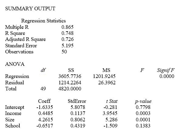-Referring to Table 14-4,suppose the builder wants to test whether the coefficient on School is significantly different from 0.What is the value of the relevant t-statistic?

TABLE 14-13 An econometrician is interested in evaluating the relationship of demand for building materials to mortgage rates in Los Angeles and San Francisco.He believes that the appropriate model is Y = 10 + 5X₁ + 8X₂ where X₁ = mortgage rate in % X₂ = 1 if SF,0 if LA Y = demand in $100 per capita -Referring to Table 14-13,the effect of living in San Francisco rather than Los Angeles is to increase the mean demand by an estimated ________.

TABLE 14-16 What are the factors that determine the acceleration time (in sec.)from 0 to 60 miles per hour of a car? Data on the following variables for 171 different vehicle models were collected: Accel Time: Acceleration time in sec. Cargo Vol: Cargo volume in cu.ft. HP: Horsepower MPG: Miles per gallon SUV: 1 if the vehicle model is an SUV with Coupe as the base when SUV and Sedan are both 0 Sedan: 1 if the vehicle model is a sedan with Coupe as the base when SUV and Sedan are both 0 The regression results using acceleration time as the dependent variable and the remaining variables as the independent variables are presented below. The various residual plots are as shown below. The coefficients of partial determination (R )of each of the 5 predictors are,respectively,0.0380,0.4376,0.0248,0.0188,and 0.0312. The coefficient of multiple determination for the regression model using each of the 5 variables Xⱼ as the dependent variable and all other X variables as independent variables (R )are,respectively,0.7461,0.5676,0.6764,0.8582,0.6632. -Referring to 14-16,there is enough evidence to conclude that Cargo Vol makes a significant contribution to the regression model in the presence of the other independent variables at a 5% level of significance.

TABLE 14-7 The department head of the accounting department wanted to see if she could predict the GPA of students using the number of course units (credits)and total SAT scores of each.She takes a sample of students and generates the following Microsoft Excel output: 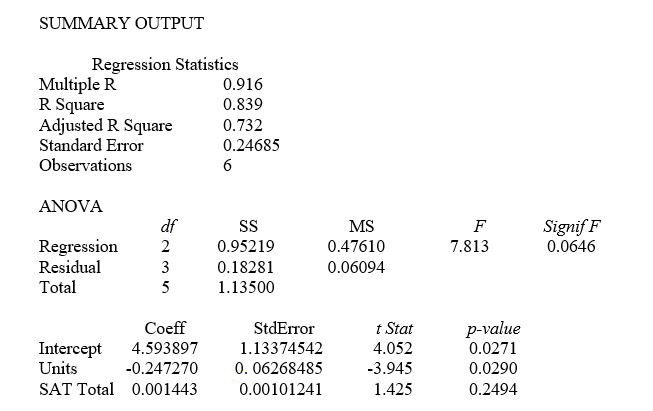-Referring to Table 14-7,the value of the adjusted coefficient of multiple determination,r²ₐdⱼ,is ________.

TABLE 14-8 A financial analyst wanted to examine the relationship between salary (in $1,000)and 4 variables: age (X₁ = Age),experience in the field (X₂ = Exper),number of degrees (X₃ = Degrees),and number of previous jobs in the field (X₄ = Prevjobs).He took a sample of 20 employees and obtained the following Microsoft Excel output: 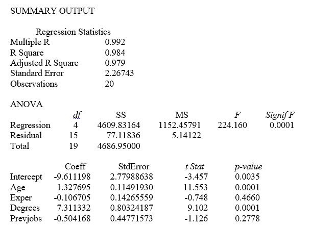-Referring to Table 14-8,the analyst wants to use an F-test to test H₀: β₁ = β₂ = β₃ = β₄ = 0.The appropriate alternative hypothesis is ________.

TABLE 14-5 A microeconomist wants to determine how corporate sales are influenced by capital and wage spending by companies.She proceeds to randomly select 26 large corporations and record information in millions of dollars.The Microsoft Excel output below shows results of this multiple regression. 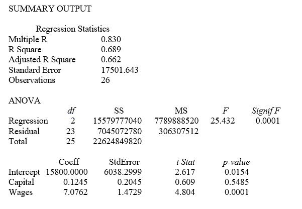-Referring to Table 14-5,what are the predicted sales (in millions of dollars)for a company spending $100 million on capital and $100 million on wages?

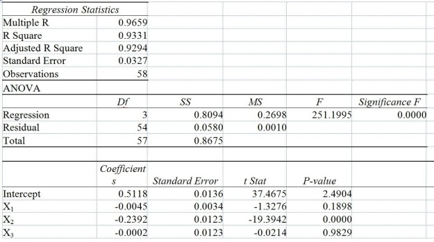
TABLE 14-15 The superintendent of a school district wanted to predict the percentage of students passing a sixth-grade proficiency test.She obtained the data on percentage of students passing the proficiency test (% Passing),daily mean of the percentage of students attending class (% Attendance),mean teacher salary in dollars (Salaries),and instructional spending per pupil in dollars (Spending)of 47 schools in the state. Following is the multiple regression output with Y = % Passing as the dependent variable,X₁ = % Attendance,X₂= Salaries and X₃= Spending: 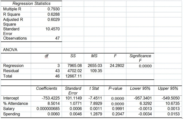-Referring to Table 14-15,estimate the mean percentage of students passing the proficiency test for all the schools that have a daily mean of 95% of students attending class,an mean teacher salary of 40,000 dollars,and an instructional spending per pupil of 2,000 dollars.

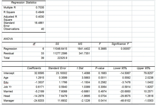
TABLE 14-17 Given below are results from the regression analysis where the dependent variable is the number of weeks a worker is unemployed due to a layoff (Unemploy)and the independent variables are the age of the worker (Age),the number of years of education received (Edu),the number of years at the previous job (Job Yr),a dummy variable for marital status (Married: 1 = married,0 = otherwise),a dummy variable for head of household (Head: 1 = yes,0 = no)and a dummy variable for management position (Manager: 1 = yes,0 = no).We shall call this Model 1.The coefficients of partial determination (R )of each of the 6 predictors are,respectively,0.2807,0.0386,0.0317,0.0141,0.0958,and 0.1201. 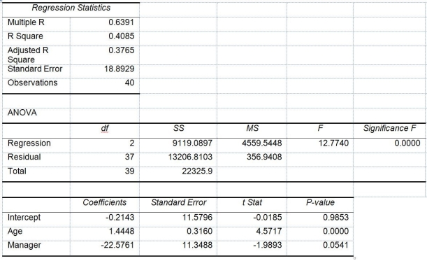Model 2 is the regression analysis where the dependent variable is Unemploy and the independent variables are Age and Manager.The results of the regression analysis are given below: -Referring to Table 14-17 Model 1,________ of the variation in the number of weeks a worker is unemployed due to a layoff can be explained by whether the worker is head of household while controlling for the other independent variables.

TABLE 14-19 The marketing manager for a nationally franchised lawn service company would like to study the characteristics that differentiate home owners who do and do not have a lawn service.A random sample of 30 home owners located in a suburban area near a large city was selected; 15 did not have a lawn service (code 0)and 15 had a lawn service (code 1).Additional information available concerning these 30 home owners includes family income (Income,in thousands of dollars),lawn size (Lawn Size,in thousands of square feet),attitude toward outdoor recreational activities (Atitude 0 = unfavorable,1 = favorable),number of teenagers in the household (Teenager),and age of the head of the household (Age). The Minitab output is given below: 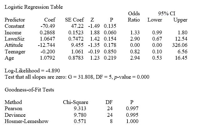-Referring to Table 14-19,the null hypothesis that the model is a good-fitting model cannot be rejected when allowing for a 5% probability of making a type I error.

TABLE 14-17 Given below are results from the regression analysis where the dependent variable is the number of weeks a worker is unemployed due to a layoff (Unemploy)and the independent variables are the age of the worker (Age),the number of years of education received (Edu),the number of years at the previous job (Job Yr),a dummy variable for marital status (Married: 1 = married,0 = otherwise),a dummy variable for head of household (Head: 1 = yes,0 = no)and a dummy variable for management position (Manager: 1 = yes,0 = no).We shall call this Model 1.The coefficients of partial determination (R )of each of the 6 predictors are,respectively,0.2807,0.0386,0.0317,0.0141,0.0958,and 0.1201. Model 2 is the regression analysis where the dependent variable is Unemploy and the independent variables are Age and Manager.The results of the regression analysis are given below: -Referring to Table 14-17 Model 1,what is the p-value of the test statistic when testing whether being married or not makes a difference in the mean number of weeks a worker is unemployed due to a layoff while holding constant the effect of all the other independent variables?

TABLE 14-4 A real estate builder wishes to determine how house size (House)is influenced by family income (Income),family size (Size),and education of the head of household (School).House size is measured in hundreds of square feet,income is measured in thousands of dollars,and education is in years.The builder randomly selected 50 families and ran the multiple regression.Microsoft Excel output is provided below: -Referring to Table 14-4,the observed value of the F-statistic is missing from the printout.What are the degrees of freedom for this F-statistic?

TABLE 14-15 The superintendent of a school district wanted to predict the percentage of students passing a sixth-grade proficiency test.She obtained the data on percentage of students passing the proficiency test (% Passing),daily mean of the percentage of students attending class (% Attendance),mean teacher salary in dollars (Salaries),and instructional spending per pupil in dollars (Spending)of 47 schools in the state. Following is the multiple regression output with Y = % Passing as the dependent variable,X₁ = % Attendance,X₂= Salaries and X₃= Spending: -Referring to Table 14-15,which of the following is a correct statement?

A regression had the following results: SST = 102.55,SSE = 82.04.It can be said that 20.0% of the variation in the dependent variable is explained by the independent variables in the regression.

TABLE 14-12 As a project for his business statistics class,a student examined the factors that determined parking meter rates throughout the campus area.Data were collected for the price per hour of parking,blocks to the quadrangle,and one of the three jurisdictions: on campus,in downtown and off campus,or outside of downtown and off campus.The population regression model hypothesized is Yᵢ = α + β₁X₁ᵢ + β₂X₂ᵢ + β₃X₃ᵢ + ε where Y is the meter price X₁ is the number of blocks to the quad X₂ is a dummy variable that takes the value 1 if the meter is located in downtown and off campus and the value 0 otherwise X₃ is a dummy variable that takes the value 1 if the meter is located outside of downtown and off campus,and the value 0 otherwise The following Excel results are obtained. -Referring to Table 14-12,what is the correct interpretation for the estimated coefficient for X₂?

TABLE 14-19 The marketing manager for a nationally franchised lawn service company would like to study the characteristics that differentiate home owners who do and do not have a lawn service.A random sample of 30 home owners located in a suburban area near a large city was selected; 15 did not have a lawn service (code 0)and 15 had a lawn service (code 1).Additional information available concerning these 30 home owners includes family income (Income,in thousands of dollars),lawn size (Lawn Size,in thousands of square feet),attitude toward outdoor recreational activities (Atitude 0 = unfavorable,1 = favorable),number of teenagers in the household (Teenager),and age of the head of the household (Age). The Minitab output is given below: -Referring to Table 14-19,there is not enough evidence to conclude that LawnSize makes a significant contribution to the model in the presence of the other independent variables at a 0.05 level of significance.

TABLE 14-17 Given below are results from the regression analysis where the dependent variable is the number of weeks a worker is unemployed due to a layoff (Unemploy)and the independent variables are the age of the worker (Age),the number of years of education received (Edu),the number of years at the previous job (Job Yr),a dummy variable for marital status (Married: 1 = married,0 = otherwise),a dummy variable for head of household (Head: 1 = yes,0 = no)and a dummy variable for management position (Manager: 1 = yes,0 = no).We shall call this Model 1.The coefficients of partial determination (R )of each of the 6 predictors are,respectively,0.2807,0.0386,0.0317,0.0141,0.0958,and 0.1201. Model 2 is the regression analysis where the dependent variable is Unemploy and the independent variables are Age and Manager.The results of the regression analysis are given below: -Referring to Table 14-17 Model 1,what are the lower and upper limits of the 95% confidence interval estimate for the effect of a one year increase in education received on the mean number of weeks a worker is unemployed due to a layoff after taking into consideration the effect of all the other independent variables?