Exam 15: Time-Series Forecasting and Index Numbers
Exam 1: Introduction to Statistics130 Questions
Exam 2: Charts and Graphs94 Questions
Exam 3: Descriptive Statistics105 Questions
Exam 4: Probability122 Questions
Exam 5: Discrete Distributions75 Questions
Exam 6: Continuous Distributions107 Questions
Exam 7: Sampling and Sampling Distributions101 Questions
Exam 8: Statistical Inference: Estimation for Single Populations75 Questions
Exam 9: Statistical Inference: Hypothesis Testing for Single Populations73 Questions
Exam 10: Statistical Inferences About Two Populations73 Questions
Exam 11: Analysis of Variance and Design of Experiments75 Questions
Exam 12: Simple Regression Analysis and Correlation75 Questions
Exam 13: Multiple Regression Analysis75 Questions
Exam 14: Building Multiple Regression Models75 Questions
Exam 15: Time-Series Forecasting and Index Numbers74 Questions
Exam 16: Analysis of Categorical Data74 Questions
Exam 17: Nonparametric Statistics79 Questions
Exam 18: Statistical Quality Control75 Questions
Exam 19: Decision Analysis77 Questions
Select questions type
When a trucking firm uses the number of shipments for January of the previous year as the forecast for January next year, it is using a naïve forecasting model.
Free
(True/False)
4.8/5  (25)
(25)
Correct Answer: Verified
True
Naïve forecasting models have no useful applications because they do not take into account data trend, cyclical effects or seasonality.
Free
(True/False)
4.9/5 (29)
Correct Answer:Verified
False
Analysis of data for an autoregressive forecasting model produced the following tables: 
 The actual values of this time series, y, were 228, 54, and 191 for May, June, and July, respectively.The forecast value predicted by the model for July is ___.
Free
(Multiple Choice)
4.8/5 (24)
Correct Answer:Verified
C
Two popular general categories of smoothing techniques are averaging models and exponential models.
(True/False)
4.8/5 (31)
Use of a smoothing constant value less than 0.5 in an exponential smoothing model gives more weight to ___.
(Multiple Choice)
4.8/5 (30)
The ratios of "actuals to moving averages" (seasonal indexes)for a time series are presented in the following table as percentages:  The final (completely adjusted)estimate of the seasonal index for Q1 is ___.
(Multiple Choice)
4.9/5 (42)
Using 2019 as the base year, the 2018 value of the Paasche Price Index is ___. 
(Multiple Choice)
4.8/5 (27)
The following graph of a time-series data suggests a ___ trend. 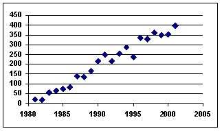
(Multiple Choice)
4.8/5 (39)
The following graph of time-series data suggests a ___ trend. 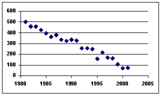
(Multiple Choice)
4.9/5 (31)
Using a three-month moving average (with weights of 6, 3, and 1 for the most current value, next most current value and oldest value, respectively), the forecast value for October made at the end of September in the following time series would be___. 
(Multiple Choice)
4.8/5 (26)
Fitting a linear trend to 36 monthly data points (January 2017 = 1, February 2017 = 2, March 2017 = 3, etc.)produced the following tables: 
 The projected trend value for January 2020 is ___.
(Multiple Choice)
4.7/5 (32)
In exponential smoothing models, the value of the smoothing constant may be any number between ___.
(Multiple Choice)
5.0/5 (29)
Use of a smoothing constant value greater than 0.5 in an exponential smoothing model gives more weight to ___.
(Multiple Choice)
4.9/5 (39)
One of the main techniques for isolating the effects of seasonality is decomposition.
(True/False)
4.9/5 (34)
Jim Royo, manager of Billings Building Supply (BBS), wants to develop a model to forecast BBS's monthly sales (in $1,000's).He selects the dollar value of residential building permits (in $10,000)as the predictor variable.An analysis of the data yielded the following tables: 
 Using = 0.05 the critical value of the Durbin-Watson statistic, dU, is ___.
(Multiple Choice)
4.9/5 (31)
Using 2016 as the base year, the 2018 value of a simple price index for the following price data is ___. 
(Multiple Choice)
4.9/5 (31)
One of the ways to overcome the autocorrelation problem in a regression forecasting model is to transform the variables by taking the first-order differences.
(True/False)
4.9/5 (33)
A time series with forecast values and error terms is presented in the following table.The mean error (ME)for this forecast is ___. 
(Multiple Choice)
4.8/5 (31)
Using a three-month moving average, the forecast value for November in the following time series is ___. 
(Multiple Choice)
4.9/5 (42)
The forecast value for September was 10.6 and the actual value turned out to be 7.Using exponential smoothing with = 0.20, the forecast value for October would be ___.
(Multiple Choice)
4.8/5 (30)
Filters
- Essay(0)
- Multiple Choice(0)
- Short Answer(0)
- True False(0)
- Matching(0)