Exam 10: Two-Sample Tests and One-Way ANOVA

In testing for differences between the means of two independent populations, the null hypothesis is:

TABLE 10-3 A real estate company is interested in testing whether the mean time that families in Gotham have been living in their current homes is less than families in Metropolis. Assume that the two population variances are equal. A random sample of 100 families from Gotham and a random sample of 150 families in Metropolis yield the following data on length of residence in current homes. Gotham: G = 35 months, SG2 = 900 Metropolis: M = 50 months, SM2 = 1,050 -Referring to Table 10-3, what is the 95% confidence interval estimate for the difference in the two means?

TABLE 10-17 A realtor wants to compare the mean sales-to-appraisal ratios of residential properties sold in four neighborhoods (A, B, C, and D). Four properties are randomly selected from each neighborhood and the ratios recorded for each, as shown below. A: 1.2, 1.1, 0.9, 0.4 C: 1.0, 1.5, 1.1, 1.3 B: 2.5, 2.1, 1.9, 1.6 D: 0.8, 1.3, 1.1, 0.7 Interpret the results of the analysis summarized in the following table: 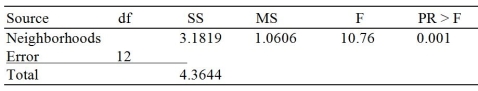-Referring to Table 10-17, the p-value of the test statistic for Levene's test for homogeneity of variances is ________.

The MSE must always be positive.

The t test for the difference between the means of two independent populations assumes that the respective

If you wish to determine whether there is evidence that the proportion of items of interest is higher in group 1 than in group 2, the appropriate test to use is

If you are comparing the mean sales among three different brands you are dealing with a three-way ANOVA design.

TABLE 10-18 As part of an evaluation program, a sporting goods retailer wanted to compare the downhill coasting speeds of four brands of bicycles. She took three of each brand and determined their maximum downhill speeds. The results are presented in miles per hour in the table below 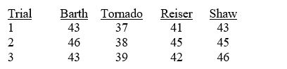-Referring to Table 10-18, the test is valid only if the population of speeds is normally distributed.

If we are testing for the difference between the means of two related populations with samples of n₁ = 20 and n₂ = 20, the number of degrees of freedom is equal to

TABLE 10-18 As part of an evaluation program, a sporting goods retailer wanted to compare the downhill coasting speeds of four brands of bicycles. She took three of each brand and determined their maximum downhill speeds. The results are presented in miles per hour in the table below -Referring to Table 10-18, the decision made implies that all four means are significantly different.

TABLE 10-1 Are Japanese managers more motivated than American managers? A randomly selected group of each were administered the Sarnoff Survey of Attitudes Toward Life (SSATL), which measures motivation for upward mobility. The SSATL scores are summarized below. 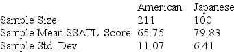-Referring to Table 10-1, what is the value of the test statistic?

TABLE 10-11 The dean of a college is interested in the proportion of graduates from his college who have a job offer on graduation day. He is particularly interested in seeing if there is a difference in this proportion for accounting and economics majors. In a random sample of 100 of each type of major at graduation, he found that 65 accounting majors and 52 economics majors had job offers. If the accounting majors are designated as "Group 1" and the economics majors are designated as "Group 2," perform the appropriate hypothesis test using a level of significance of 0.05. -Referring to Table 10-11, construct a 95% confidence interval estimate of the difference in proportion between accounting majors and economic majors who have a job offer on graduation day.

TABLE 10-8 A few years ago, Pepsi invited consumers to take the "Pepsi Challenge." Consumers were asked to decide which of two sodas, Coke or Pepsi, they preferred in a blind taste test. Pepsi was interested in determining what factors played a role in people's taste preferences. One of the factors studied was the gender of the consumer. Below are the results of analyses comparing the taste preferences of men and women with the proportions depicting preference for Pepsi. Males: n = 109, pM = 0.422018 Females: n = 52, pF = 0.25 pM - pF = 0.172018 Z = 2.11825 -Referring to Table 10-8, construct a 90% confidence interval estimate of the difference between the proportion of males and females who prefer Pepsi.

TABLE 10-8 A few years ago, Pepsi invited consumers to take the "Pepsi Challenge." Consumers were asked to decide which of two sodas, Coke or Pepsi, they preferred in a blind taste test. Pepsi was interested in determining what factors played a role in people's taste preferences. One of the factors studied was the gender of the consumer. Below are the results of analyses comparing the taste preferences of men and women with the proportions depicting preference for Pepsi. Males: n = 109, pM = 0.422018 Females: n = 52, pF = 0.25 pM - pF = 0.172018 Z = 2.11825 -Referring to Table 10-8, suppose Pepsi wanted to test to determine if the males preferred Pepsi more than the females. Using the test statistic given, compute the appropriate p-value for the test.

TABLE 10-20 A hotel chain has identically sized resorts in five locations. The data that follow resulted from analyzing the hotel occupancies on randomly selected days in the five locations. 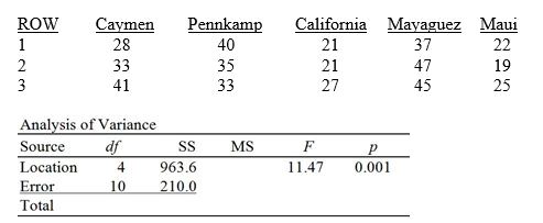-Referring to Table 10-20, the total variation or SST is ________.

TABLE 10-20 A hotel chain has identically sized resorts in five locations. The data that follow resulted from analyzing the hotel occupancies on randomly selected days in the five locations. -Referring to Table 10-20, the among-group variation or SSA is ________.

TABLE 10-17 A realtor wants to compare the mean sales-to-appraisal ratios of residential properties sold in four neighborhoods (A, B, C, and D). Four properties are randomly selected from each neighborhood and the ratios recorded for each, as shown below. A: 1.2, 1.1, 0.9, 0.4 C: 1.0, 1.5, 1.1, 1.3 B: 2.5, 2.1, 1.9, 1.6 D: 0.8, 1.3, 1.1, 0.7 Interpret the results of the analysis summarized in the following table: -Referring to Table 10-17, what should be the conclusion for the Levene's test for homogeneity of variances at a 5% level of significance?

TABLE 10-7 A buyer for a manufacturing plant suspects that his primary supplier of raw materials is overcharging. In order to determine if his suspicion is correct, he contacts a second supplier and asks for the prices on various identical materials. He wants to compare these prices with those of his primary supplier. The data collected is presented in the table below, with some summary statistics presented (all of these might not be necessary to answer the questions which follow). The buyer believes that the differences are normally distributed and will use this sample to perform an appropriate test at a level of significance of 0.01. 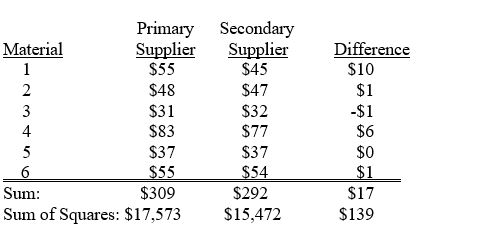-Referring to Table 10-7, the buyer should decide that the primary supplier is

TABLE 10-19 An agronomist wants to compare the crop yield of 3 varieties of chickpea seeds. She plants 15 fields, 5 with each variety. She then measures the crop yield in bushels per acre. Treating this as a completely randomized design, the results are presented in the table that follows. 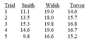-Referring to Table 10-19, the within-group variation or SSW is ________.

TABLE 10-14 The use of preservatives by food processors has become a controversial issue. Suppose two preservatives are extensively tested and determined safe for use in meats. A processor wants to compare the preservatives for their effects on retarding spoilage. Suppose 15 cuts of fresh meat are treated with preservative I and 15 are treated with preservative II, and the number of hours until spoilage begins is recorded for each of the 30 cuts of meat. The results are summarized in the table below. Preservative I Preservative II I = 106.4 hours II= 96.54 hours SI = 10.3 hours SII = 13.4 hours -Referring to Table 10-14, what is the critical value for testing if the population variances differ for preservatives I and II at the 5% level of significance?