Exam 10: Two-Sample Tests and One-Way ANOVA

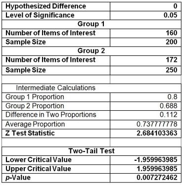
TABLE 10-9 The following Microsoft Excel output contains the results of a test to determine whether the proportions of satisfied customers at two resorts are the same or different. -Referring to Table 10-9, allowing for 1% probability of committing a Type I error, what are the decision and conclusion on testing whether there is any difference in the proportions of satisfied customers in the two resorts?

TABLE 10-10 A corporation randomly selects 150 salespeople and finds that 66% who have never taken a self-improvement course would like such a course. The firm did a similar study 10 years ago in which 60% of a random sample of 160 salespeople wanted a self-improvement course. The groups are assumed to be independent random samples. Let π1 and π2 represent the true proportion of workers who would like to attend a self-improvement course in the recent study and the past study, respectively. -Referring to Table 10-10, what is/are the critical value(s)when testing whether the current population proportion is higher than before if α = 0.05?

TABLE 10-15 The table below presents the summary statistics for the starting annual salaries (in thousands of dollars) for individuals entering the public accounting and financial planning professions. Sample 1 (public accounting): 1 = 60.35, S1 = 3.25, n1 = 12 Sample 2 (financial planning): 2 = 58.20, S2 = 2.48, n2 = 14 Test whether the mean starting annual salaries for individuals entering the public accounting professions is higher than that of financial planning, assuming that the two population variances are the same. -Referring to Table 10-15, state the null and alternative hypotheses for testing whether there is evidence of a difference in the variances of the starting annual salaries.

TABLE 10-7 A buyer for a manufacturing plant suspects that his primary supplier of raw materials is overcharging. In order to determine if his suspicion is correct, he contacts a second supplier and asks for the prices on various identical materials. He wants to compare these prices with those of his primary supplier. The data collected is presented in the table below, with some summary statistics presented (all of these might not be necessary to answer the questions which follow). The buyer believes that the differences are normally distributed and will use this sample to perform an appropriate test at a level of significance of 0.01. 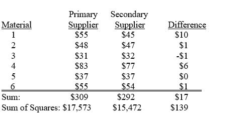-Referring to Table 10-7, what is the 95% confidence interval estimate for the mean difference in prices?

TABLE 10-12 A quality control engineer is in charge of the manufacture of computer disks. Two different processes can be used to manufacture the disks. He suspects that the Kohler method produces a greater proportion of defects than the Russell method. He samples 150 of the Kohler and 200 of the Russell disks and finds that 27 and 18 of them, respectively, are defective. If Kohler is designated as "Group 1" and Russell is designated as "Group 2," perform the appropriate test at a level of significance of 0.01. -Referring to Table 10-12, the same decision would be made if this had been a two-tail test at a level of significance of 0.01.

TABLE 10-19 An agronomist wants to compare the crop yield of 3 varieties of chickpea seeds. She plants 15 fields, 5 with each variety. She then measures the crop yield in bushels per acre. Treating this as a completely randomized design, the results are presented in the table that follows. -Referring to Table 10-19, the among-group variation or SSA is ________.

The F distribution is symmetric.

TABLE 10-15 The table below presents the summary statistics for the starting annual salaries (in thousands of dollars) for individuals entering the public accounting and financial planning professions. Sample 1 (public accounting): 1 = 60.35, S1 = 3.25, n1 = 12 Sample 2 (financial planning): 2 = 58.20, S2 = 2.48, n2 = 14 Test whether the mean starting annual salaries for individuals entering the public accounting professions is higher than that of financial planning, assuming that the two population variances are the same. -Referring to Table 10-15, which of the following represents the relevant hypotheses tested?

TABLE 10-8 A few years ago, Pepsi invited consumers to take the "Pepsi Challenge." Consumers were asked to decide which of two sodas, Coke or Pepsi, they preferred in a blind taste test. Pepsi was interested in determining what factors played a role in people's taste preferences. One of the factors studied was the gender of the consumer. Below are the results of analyses comparing the taste preferences of men and women with the proportions depicting preference for Pepsi. Males: n = 109, pM = 0.422018 Females: n = 52, pF = 0.25 pM - pF = 0.172018 Z = 2.11825 -Referring to Table 10-8, suppose that the two-tail p-value was really 0.0734. State the proper conclusion.

TABLE 10-14 The use of preservatives by food processors has become a controversial issue. Suppose two preservatives are extensively tested and determined safe for use in meats. A processor wants to compare the preservatives for their effects on retarding spoilage. Suppose 15 cuts of fresh meat are treated with preservative I and 15 are treated with preservative II, and the number of hours until spoilage begins is recorded for each of the 30 cuts of meat. The results are summarized in the table below. Preservative I Preservative II I = 106.4 hours II= 96.54 hours SI = 10.3 hours SII = 13.4 hours -Referring to Table 10-14, state the null and alternative hypotheses for testing if the population variances differ for preservatives I and II.

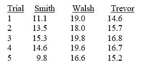
TABLE 10-16 An airline wants to select a computer software package for its reservation system. Four software packages (1, 2, 3, and 4) are commercially available. The airline will choose the package that bumps as few passengers as possible during a month. An experiment is set up in which each package is used to make reservations for 5 randomly selected weeks. (A total of 20 weeks was included in the experiment.) The number of passengers bumped each week is obtained, which gives rise to the following Microsoft Excel output: 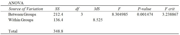-Referring to Table 10-16, at a significance level of 1%,

TABLE 10-20 A hotel chain has identically sized resorts in five locations. The data that follow resulted from analyzing the hotel occupancies on randomly selected days in the five locations. 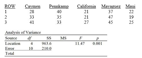-Referring to Table 10-20, if a level of significance of 0.05 is chosen, the decision made indicates that at least two of the five locations have different mean occupancy rates.

TABLE 10-2 A researcher randomly sampled 30 graduates of an MBA program and recorded data concerning their starting salaries. Of primary interest to the researcher was the effect of gender on starting salaries. The result of the pooled-variance t test of the mean salaries of the females (Population 1) and males (Population 2) in the sample is given below. 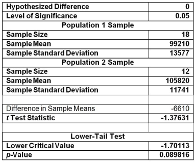-Referring to Table 10-2, what is the 90% confidence interval estimate for the difference between two means?

TABLE 10-20 A hotel chain has identically sized resorts in five locations. The data that follow resulted from analyzing the hotel occupancies on randomly selected days in the five locations. -Referring to Table 10-20, what is the p-value of the test statistic for Levene's test for homogeneity of variances?

TABLE 10-9 The following Microsoft Excel output contains the results of a test to determine whether the proportions of satisfied customers at two resorts are the same or different. -Referring to Table 10-9, if you want to test the claim that "Resort 1 (Group 1)has a higher proportion of satisfied customers compared to Resort 2 (Group 2)", the p-value of the test will be ________.

TABLE 10-15 The table below presents the summary statistics for the starting annual salaries (in thousands of dollars) for individuals entering the public accounting and financial planning professions. Sample 1 (public accounting): 1 = 60.35, S1 = 3.25, n1 = 12 Sample 2 (financial planning): 2 = 58.20, S2 = 2.48, n2 = 14 Test whether the mean starting annual salaries for individuals entering the public accounting professions is higher than that of financial planning, assuming that the two population variances are the same. -Referring to Table 10-15, suppose α = 0.01. Which of the following represents the correct conclusion?

A completely randomized design

TABLE 10-20 A hotel chain has identically sized resorts in five locations. The data that follow resulted from analyzing the hotel occupancies on randomly selected days in the five locations. -Referring to Table 10-20, what is the critical value of Levene's test for homogeneity of variances at a 5% level of significance?

In testing for the differences between the means of two related populations, the ________ hypothesis is the hypothesis of "no differences."

TABLE 10-10 A corporation randomly selects 150 salespeople and finds that 66% who have never taken a self-improvement course would like such a course. The firm did a similar study 10 years ago in which 60% of a random sample of 160 salespeople wanted a self-improvement course. The groups are assumed to be independent random samples. Let π1 and π2 represent the true proportion of workers who would like to attend a self-improvement course in the recent study and the past study, respectively. -Referring to Table 10-10, what is/are the critical value(s)when testing whether population proportions are different if α = 0.10?