Exam 25: Multiple and Logistic Regression
Exam 1: Picturing Distributions With Graphs38 Questions
Exam 2: Describing Quantitative Distributions With Numbers42 Questions
Exam 3: Scatterplots and Correlation42 Questions
Exam 4: Regression41 Questions
Exam 5: Two-Way Tables35 Questions
Exam 6: Samples and Observational Studies34 Questions
Exam 7: Designing Experiments40 Questions
Exam 8: Essential Probability Rules58 Questions
Exam 9: Independence and Conditional Probabilities38 Questions
Exam 10: The Normal Distributions43 Questions
Exam 11: Discrete Probability Distributions43 Questions
Exam 12: Sampling Distributions48 Questions
Exam 13: Introduction to Inference48 Questions
Exam 14: Exercises44 Questions
Exam 15: Inference About a Population Mean44 Questions
Exam 16: Comparing Two Means40 Questions
Exam 17: Inference About a Population Proportion39 Questions
Exam 18: Comparing Two Proportions47 Questions
Exam 19: The Chi-Square Test for Goodness of Fit40 Questions
Exam 20: The Chi-Square Test for Two-Way Tables42 Questions
Exam 21: Inference for Regression45 Questions
Exam 22: One-Way Analysis of Variance: Comparing Several Means40 Questions
Exam 23: More About Analysis of Variance: Follow-Up Tests and Two-Way Anova39 Questions
Exam 24: Nonparametric Tests41 Questions
Exam 25: Multiple and Logistic Regression28 Questions
Select questions type
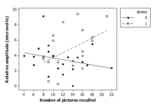
Researchers investigated the effects of acute stress on emotional picture processing and recall by randomly assigning 40 adult males to receive either a stressful cold stimulus or a neutral warm stimulus before viewing pictures. The researchers computed the relative brainwave amplitude (in microvolts, μV) for each subject viewing unpleasant versus neutral pictures. They also recorded how many pictures the subjects were able to recall 24 hours later. The data are displayed in the following scatterplot.
μ  The following model is proposed for predicting the brainwave relative amplitude ("amplitude") from the number of images recalled ("recall"), the indicator variable reflecting the nature of the stimulus ("stress"), and an interaction term ("recall*stress"):
Amplitudei = β0 + β1 (recalli) + β2 (stressi) + β3 (recall*stressi) + εi
Where the deviations εi are assumed to be independent and Normally distributed with mean 0 and standard deviation σ. This model was fit to the sample of 40 adult males. The following results summarize the least-squares regression fit of this model:
Predictor Coef SE Coef Constant 4.795 1.329 recall -0.1139 0.1069 stress -4.262 2.205 recall 0.4337 0.1677 =2.13946 R-Sq =22.8\%
Analysis of Variance Source DF SS MS Regression 3 48.788 16.263 Residual Error 36 164.783 4.577 Total 39 213.571 Suppose we wish use the ANOVA F test to test the following hypotheses:
H0: β1 = β2 = β3 = 0
Hα: At least one of β1 or β2 or β3 is not 0
What is the value of the F statistic for these hypotheses?
The following model is proposed for predicting the brainwave relative amplitude ("amplitude") from the number of images recalled ("recall"), the indicator variable reflecting the nature of the stimulus ("stress"), and an interaction term ("recall*stress"):
Amplitudei = β0 + β1 (recalli) + β2 (stressi) + β3 (recall*stressi) + εi
Where the deviations εi are assumed to be independent and Normally distributed with mean 0 and standard deviation σ. This model was fit to the sample of 40 adult males. The following results summarize the least-squares regression fit of this model:
Predictor Coef SE Coef Constant 4.795 1.329 recall -0.1139 0.1069 stress -4.262 2.205 recall 0.4337 0.1677 =2.13946 R-Sq =22.8\%
Analysis of Variance Source DF SS MS Regression 3 48.788 16.263 Residual Error 36 164.783 4.577 Total 39 213.571 Suppose we wish use the ANOVA F test to test the following hypotheses:
H0: β1 = β2 = β3 = 0
Hα: At least one of β1 or β2 or β3 is not 0
What is the value of the F statistic for these hypotheses?
Free
(Multiple Choice)
4.9/5  (41)
(41)
Correct Answer: Verified
B
Researchers investigated the effects of acute stress on emotional picture processing and recall by randomly assigning 40 adult males to receive either a stressful cold stimulus or a neutral warm stimulus before viewing pictures. The researchers computed the relative brainwave amplitude (in microvolts, μV) for each subject viewing unpleasant versus neutral pictures. They also recorded how many pictures the subjects were able to recall 24 hours later. The data are displayed in the following scatterplot.
 The following model is proposed for predicting the brainwave relative amplitude ("amplitude") from the number of images recalled ("recall"), the indicator variable reflecting the nature of the stimulus ("stress"), and an interaction term ("recall*stress"):
Amplitudei = β0 + β1 (recalli) + β2 (stressi) + β3 (recall*stressi) + εi
Where the deviations εi are assumed to be independent and Normally distributed with mean 0 and standard deviation σ. This model was fit to the sample of 40 adult males. The following results summarize the least-squares regression fit of this model:
Predictor Coef SE Coef Constant 4.795 1.329 recall -0.1139 0.1069 stress -4.262 2.205 recall stress 0.4337 0.1677 =2.13946 R-Sq =22.8\%
Analysis of Variance Source DF SS MS Regression 3 48.788 16.263 Residual Error 36 164.783 4.577 Total 39 213.571 The interaction term in this model is statistically significant at the 0.05 level. Given this and the scatterplot provided, what should you conclude?
The following model is proposed for predicting the brainwave relative amplitude ("amplitude") from the number of images recalled ("recall"), the indicator variable reflecting the nature of the stimulus ("stress"), and an interaction term ("recall*stress"):
Amplitudei = β0 + β1 (recalli) + β2 (stressi) + β3 (recall*stressi) + εi
Where the deviations εi are assumed to be independent and Normally distributed with mean 0 and standard deviation σ. This model was fit to the sample of 40 adult males. The following results summarize the least-squares regression fit of this model:
Predictor Coef SE Coef Constant 4.795 1.329 recall -0.1139 0.1069 stress -4.262 2.205 recall stress 0.4337 0.1677 =2.13946 R-Sq =22.8\%
Analysis of Variance Source DF SS MS Regression 3 48.788 16.263 Residual Error 36 164.783 4.577 Total 39 213.571 The interaction term in this model is statistically significant at the 0.05 level. Given this and the scatterplot provided, what should you conclude?
Free
(Multiple Choice)
4.9/5 (43)
Correct Answer:Verified
A
Researchers investigated the effects of acute stress on emotional picture processing and recall by randomly assigning 40 adult males to receive either a stressful cold stimulus or a neutral warm stimulus before viewing pictures. The researchers computed the relative brainwave amplitude (in microvolts, μV) for each subject viewing unpleasant versus neutral pictures. They also recorded how many pictures the subjects were able to recall 24 hours later. The data are displayed in the following scatterplot.
 The following model is proposed for predicting the brainwave relative amplitude ("amplitude") from the number of images recalled ("recall"), the indicator variable reflecting the nature of the stimulus ("stress"), and an interaction term ("recall*stress"):
Amplitudei = β0 + β1 (recalli) + β2 (stressi) + β3 (recall*stressi) + εi
Where the deviations εi are assumed to be independent and Normally distributed with mean 0 and standard deviation σ. This model was fit to the sample of 40 adult males. The following results summarize the least-squares regression fit of this model:
Predictor Coef SE Coef Constant 4.795 1.329 recall -0.1139 0.1069 stress -4.262 2.205 stress 0.4337 0.1677 =2.13946 R-Sq =22.8\%
Analysis of Variance Source DF SS MS Regression 3 48.788 16.263 Residual Error 36 164.783 4.577 Total 39 213.571 Based on the software output provided, what is the equation of the regression model when a stressful stimulus is received (indicator variable stress = 1)?
The following model is proposed for predicting the brainwave relative amplitude ("amplitude") from the number of images recalled ("recall"), the indicator variable reflecting the nature of the stimulus ("stress"), and an interaction term ("recall*stress"):
Amplitudei = β0 + β1 (recalli) + β2 (stressi) + β3 (recall*stressi) + εi
Where the deviations εi are assumed to be independent and Normally distributed with mean 0 and standard deviation σ. This model was fit to the sample of 40 adult males. The following results summarize the least-squares regression fit of this model:
Predictor Coef SE Coef Constant 4.795 1.329 recall -0.1139 0.1069 stress -4.262 2.205 stress 0.4337 0.1677 =2.13946 R-Sq =22.8\%
Analysis of Variance Source DF SS MS Regression 3 48.788 16.263 Residual Error 36 164.783 4.577 Total 39 213.571 Based on the software output provided, what is the equation of the regression model when a stressful stimulus is received (indicator variable stress = 1)?
Free
(Multiple Choice)
4.8/5 (35)
Correct Answer:Verified
B
Researchers investigated the effects of acute stress on emotional picture processing and recall by randomly assigning 40 adult males to receive either a stressful cold stimulus or a neutral warm stimulus before viewing pictures. The researchers computed the relative brainwave amplitude (in microvolts, μV) for each subject viewing unpleasant versus neutral pictures. They also recorded how many pictures the subjects were able to recall 24 hours later. The data are displayed in the following scatterplot.
 The following model is proposed for predicting the brainwave relative amplitude ("amplitude") from the number of images recalled ("recall"), the indicator variable reflecting the nature of the stimulus ("stress"), and an interaction term ("recall*stress"):
Amplitudei = β0 + β1 (recalli) + β2 (stressi) + β3 (recall*stressi) + εi
Where the deviations εi are assumed to be independent and Normally distributed with mean 0 and standard deviation σ. This model was fit to the sample of 40 adult males. The following results summarize the least-squares regression fit of this model:
Predictor Coef SE Coef Constant 4.795 1.329 recall -0.1139 0.1069 stress -4.262 2.205 recall stress 0.4337 0.1677 =2.13946 R-Sq =22.8\%
Analysis of Variance Source DF SS MS Regression 3 48.788 16.263 Residual Error 36 164.783 4.577 Total 39 213.571 What is a 95% confidence interval for β2, the coefficient of the indicator variable stress in this model?
The following model is proposed for predicting the brainwave relative amplitude ("amplitude") from the number of images recalled ("recall"), the indicator variable reflecting the nature of the stimulus ("stress"), and an interaction term ("recall*stress"):
Amplitudei = β0 + β1 (recalli) + β2 (stressi) + β3 (recall*stressi) + εi
Where the deviations εi are assumed to be independent and Normally distributed with mean 0 and standard deviation σ. This model was fit to the sample of 40 adult males. The following results summarize the least-squares regression fit of this model:
Predictor Coef SE Coef Constant 4.795 1.329 recall -0.1139 0.1069 stress -4.262 2.205 recall stress 0.4337 0.1677 =2.13946 R-Sq =22.8\%
Analysis of Variance Source DF SS MS Regression 3 48.788 16.263 Residual Error 36 164.783 4.577 Total 39 213.571 What is a 95% confidence interval for β2, the coefficient of the indicator variable stress in this model?
(Multiple Choice)
4.8/5 (30)
A case study enrolled case individuals with glioma (a type of brain cancer) and similar control individuals without glioma. Participants were asked whether they had been regular cell phone users for at least a year. We use logistic regression to model glioma status (1 = glioma, 0 = no glioma) as a function of regular cell phone use (1 = yes, 0 = no). Software gives the following information:
For log odds of glioma/no glioma
Predictor Coef SE Coef Constant -0.08074 0.04987 Regular use -0.02565 0.07275 What is a 95% confidence interval for the odds ratio eβ1?
(Multiple Choice)
5.0/5 (30)
Researchers investigated the effects of acute stress on emotional picture processing and recall by randomly assigning 40 adult males to receive either a stressful cold stimulus or a neutral warm stimulus before viewing pictures. The researchers computed the relative brainwave amplitude (in microvolts, μV) for each subject viewing unpleasant versus neutral pictures. They also recorded how many pictures the subjects were able to recall 24 hours later. The data are displayed in the following scatterplot.
 The following model is proposed for predicting the brainwave relative amplitude ("amplitude") from the number of images recalled ("recall"), the indicator variable reflecting the nature of the stimulus ("stress"), and an interaction term ("recall*stress"):
Amplitudei = β0 + β1 (recalli) + β2 (stressi) + β3 (recall*stressi) + εi
Where the deviations εi are assumed to be independent and Normally distributed with mean 0 and standard deviation σ. This model was fit to the sample of 40 adult males. The following results summarize the least-squares regression fit of this model:
Predictor Coef SE Coef Constant 4.795 1.329 recall -0.1139 0.1069 stress -4.262 2.205 recall stress 0.4337 0.1677 =2.13946 -=22.8\% Analysis of Variance
Source DF SS MS Regression 3 48.788 16.263 Residual Error 36 164.783 4.577 Total 39 213.571 To determine whether the number of pictures recalled affects the brainwave relative amplitude in this model, we test the hypotheses H0: β1 = 0, Ha: β1 ≠ 0 in this particular model. Using the estimates provided, what is the P-value for this test?
The following model is proposed for predicting the brainwave relative amplitude ("amplitude") from the number of images recalled ("recall"), the indicator variable reflecting the nature of the stimulus ("stress"), and an interaction term ("recall*stress"):
Amplitudei = β0 + β1 (recalli) + β2 (stressi) + β3 (recall*stressi) + εi
Where the deviations εi are assumed to be independent and Normally distributed with mean 0 and standard deviation σ. This model was fit to the sample of 40 adult males. The following results summarize the least-squares regression fit of this model:
Predictor Coef SE Coef Constant 4.795 1.329 recall -0.1139 0.1069 stress -4.262 2.205 recall stress 0.4337 0.1677 =2.13946 -=22.8\% Analysis of Variance
Source DF SS MS Regression 3 48.788 16.263 Residual Error 36 164.783 4.577 Total 39 213.571 To determine whether the number of pictures recalled affects the brainwave relative amplitude in this model, we test the hypotheses H0: β1 = 0, Ha: β1 ≠ 0 in this particular model. Using the estimates provided, what is the P-value for this test?
(Multiple Choice)
4.7/5 (30)
Tail-feather length is a sexually dimorphic trait in long-tailed finches; that is, the trait differs substantially for males and for females of the same species. A bird's size and environment might also influence tail-feather length. Researchers studied the relationship between tail-feather length (measuring the R1 central tail feather) and weight in a sample of 20 male long-tailed finches raised in an aviary and 5 male long-tailed finches caught in the wild. The data are displayed in the scatterplot below.
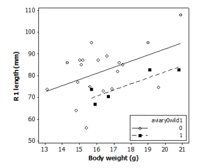 The following model is proposed for predicting the length of the R1 feather from the bird's weight and origin:
R1Lengthi = β0 + β1 (BodyWeighti) + β2 (Aviary0Wild1i) + εi
Where the deviations εi were assumed to be independent and Normally distributed with mean 0 and standard deviation σ . This model was fit to the sample of 25 male finches. The following results summarize the least-squares regression fit of this model:
Predictor Coef SE Coef Constant 35.79 16.95 BodyWeight 2.826 1.030 Aviary0Wild1 -10.453 4.996 =9.62172-=30.2\%
Analysis of Variance Source DF SS MS Regression 2 879.79 439.90 Residual Error 22 2036.71 92.58 Total 24 2916.50 Suppose we wish use the ANOVA F test to test the following hypotheses:
H0: β1 = β2 = 0
Hα: At least one of β1 or β2 is not 0
What is the P-value of this test?
The following model is proposed for predicting the length of the R1 feather from the bird's weight and origin:
R1Lengthi = β0 + β1 (BodyWeighti) + β2 (Aviary0Wild1i) + εi
Where the deviations εi were assumed to be independent and Normally distributed with mean 0 and standard deviation σ . This model was fit to the sample of 25 male finches. The following results summarize the least-squares regression fit of this model:
Predictor Coef SE Coef Constant 35.79 16.95 BodyWeight 2.826 1.030 Aviary0Wild1 -10.453 4.996 =9.62172-=30.2\%
Analysis of Variance Source DF SS MS Regression 2 879.79 439.90 Residual Error 22 2036.71 92.58 Total 24 2916.50 Suppose we wish use the ANOVA F test to test the following hypotheses:
H0: β1 = β2 = 0
Hα: At least one of β1 or β2 is not 0
What is the P-value of this test?
(Multiple Choice)
4.9/5 (35)
A study looked for a protein marker that might help predict active flare-ups in a particular chronic disease. A sample of 32 individuals with the diseases had some blood taken to determine their disease status (active flare-up or inactive) and the relative abundance of the protein marker in their blood. We use logistic regression to model disease status as a function of relative abundance. Software gives the following information:
For Log Odds of Active/Inactive
Term Estimate Std Error Intercept -6.186 2.416 tive abundance 6.229 2.651 We want to know if the slope of the logistic regression model is significant. What is the P-value for the two-sided test?
(Multiple Choice)
4.9/5 (36)
Researchers investigated the effects of acute stress on emotional picture processing and recall by randomly assigning 40 adult males to receive either a stressful cold stimulus or a neutral warm stimulus before viewing pictures. The researchers computed the relative brainwave amplitude (in microvolts, μV) for each subject viewing unpleasant versus neutral pictures. They also recorded how many pictures the subjects were able to recall 24 hours later. The data are displayed in the following scatterplot.
μ
 The following model is proposed for predicting the brainwave relative amplitude ("amplitude") from the number of images recalled ("recall"), the indicator variable reflecting the nature of the stimulus ("stress"), and an interaction term ("recall*stress"):
Amplitudei = β0 + β1 (recalli) + β2 (stressi) + β3 (recall*stressi) + εi
Where the deviations εi are assumed to be independent and Normally distributed with mean 0 and standard deviation σ. This model was fit to the sample of 40 adult males. The following results summarize the least-squares regression fit of this model:
Predictor Coef SE Coef Constant 4.795 1.329 recall -0.1139 0.1069 stress -4.262 2.205 recall* stress 0.4337 0.1677 =2.13946 R-Sq =22.8\%
Analysis of Variance Source DF SS MS Regression 3 48.788 16.263 Residual Error 36 164.783 4.577 Total 39 213.571 Based on the software output provided, what is the equation for the multiple regression model?
The following model is proposed for predicting the brainwave relative amplitude ("amplitude") from the number of images recalled ("recall"), the indicator variable reflecting the nature of the stimulus ("stress"), and an interaction term ("recall*stress"):
Amplitudei = β0 + β1 (recalli) + β2 (stressi) + β3 (recall*stressi) + εi
Where the deviations εi are assumed to be independent and Normally distributed with mean 0 and standard deviation σ. This model was fit to the sample of 40 adult males. The following results summarize the least-squares regression fit of this model:
Predictor Coef SE Coef Constant 4.795 1.329 recall -0.1139 0.1069 stress -4.262 2.205 recall* stress 0.4337 0.1677 =2.13946 R-Sq =22.8\%
Analysis of Variance Source DF SS MS Regression 3 48.788 16.263 Residual Error 36 164.783 4.577 Total 39 213.571 Based on the software output provided, what is the equation for the multiple regression model?
(Multiple Choice)
4.9/5 (33)
Researchers investigated the effects of acute stress on emotional picture processing and recall by randomly assigning 40 adult males to receive either a stressful cold stimulus or a neutral warm stimulus before viewing pictures. The researchers computed the relative brainwave amplitude (in microvolts, μV) for each subject viewing unpleasant versus neutral pictures. They also recorded how many pictures the subjects were able to recall 24 hours later. The data are displayed in the following scatterplot.
μ  The following model is proposed for predicting the brainwave relative amplitude ("amplitude") from the number of images recalled ("recall"), the indicator variable reflecting the nature of the stimulus ("stress"), and an interaction term ("recall*stress"):
Amplitudei = β0 + β1 (recalli) + β2 (stressi) + β3 (recall*stressi) + εi
Where the deviations εi are assumed to be independent and Normally distributed with mean 0 and standard deviation σ. This model was fit to the sample of 40 adult males. The following results summarize the least-squares regression fit of this model:
Predictor Coef SE Coef Constant 4.795 1.329 recall -0.1139 0.1069 stress -4.262 2.205 recall stress 0.4337 0.1677 =2.13946 R-Sq =22.8\%
Analysis of Variance Source DF SS MS Regression 3 48.788 16.263 Residual Error 36 164.783 4.577 Total 39 213.571 Here are the residual plots for this regression model:
The following model is proposed for predicting the brainwave relative amplitude ("amplitude") from the number of images recalled ("recall"), the indicator variable reflecting the nature of the stimulus ("stress"), and an interaction term ("recall*stress"):
Amplitudei = β0 + β1 (recalli) + β2 (stressi) + β3 (recall*stressi) + εi
Where the deviations εi are assumed to be independent and Normally distributed with mean 0 and standard deviation σ. This model was fit to the sample of 40 adult males. The following results summarize the least-squares regression fit of this model:
Predictor Coef SE Coef Constant 4.795 1.329 recall -0.1139 0.1069 stress -4.262 2.205 recall stress 0.4337 0.1677 =2.13946 R-Sq =22.8\%
Analysis of Variance Source DF SS MS Regression 3 48.788 16.263 Residual Error 36 164.783 4.577 Total 39 213.571 Here are the residual plots for this regression model:
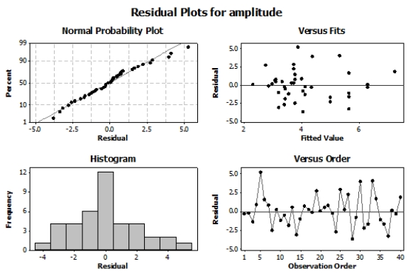 Based on the study description, the scatterplot, and the residual plots, what should you conclude?
(Multiple Choice)
4.7/5 (33)
A case study enrolled case individuals with glioma (a type of brain cancer) and similar control individuals without glioma. Participants were asked whether they had been regular cell phone users for at least a year. We use logistic regression to model glioma status (1 = glioma, 0 = no glioma) as a function of regular cell phone use (1 = yes, 0 = no). Software gives the following information:
For log odds of glioma/no glioma
Predictor Coef SE Coef Constant -0.08074 0.04987 Regular use -0.02565 0.07275 We want to know if the slope of the logistic regression model is significant. What is the P-value for the two-sided test?
(Multiple Choice)
4.7/5 (28)
Researchers investigated the effects of acute stress on emotional picture processing and recall by randomly assigning 40 adult males to receive either a stressful cold stimulus or a neutral warm stimulus before viewing pictures. The researchers computed the relative brainwave amplitude (in microvolts, μV) for each subject viewing unpleasant versus neutral pictures. They also recorded how many pictures the subjects were able to recall 24 hours later. The data are displayed in the following scatterplot.
μ  The following model is proposed for predicting the brainwave relative amplitude ("amplitude") from the number of images recalled ("recall"), the indicator variable reflecting the nature of the stimulus ("stress"), and an interaction term ("recall*stress"):
Amplitudei = β0 + β1 (recalli) + β2 (stressi) + β3 (recall*stressi) + εi
Where the deviations εi are assumed to be independent and Normally distributed with mean 0 and standard deviation σ. This model was fit to the sample of 40 adult males. The following results summarize the least-squares regression fit of this model:
Predictor Coef SE Coef Constant 4.795 1.329 recall -0.1139 0.1069 stress -4.262 2.205 recall stress 0.4337 0.1677 =2.13946 -=22.8\%
Analysis of Variance Source DF SS MS Regression 3 48.788 16.263 Residual Error 36 164.783 4.577 Total 39 213.571 What is the percent of variation in brainwave relative amplitude that can be explained by the regression model?
The following model is proposed for predicting the brainwave relative amplitude ("amplitude") from the number of images recalled ("recall"), the indicator variable reflecting the nature of the stimulus ("stress"), and an interaction term ("recall*stress"):
Amplitudei = β0 + β1 (recalli) + β2 (stressi) + β3 (recall*stressi) + εi
Where the deviations εi are assumed to be independent and Normally distributed with mean 0 and standard deviation σ. This model was fit to the sample of 40 adult males. The following results summarize the least-squares regression fit of this model:
Predictor Coef SE Coef Constant 4.795 1.329 recall -0.1139 0.1069 stress -4.262 2.205 recall stress 0.4337 0.1677 =2.13946 -=22.8\%
Analysis of Variance Source DF SS MS Regression 3 48.788 16.263 Residual Error 36 164.783 4.577 Total 39 213.571 What is the percent of variation in brainwave relative amplitude that can be explained by the regression model?
(Multiple Choice)
4.8/5 (34)
Tail-feather length is a sexually dimorphic trait in long-tailed finches; that is, the trait differs substantially for males and for females of the same species. A bird's size and environment might also influence tail-feather length. Researchers studied the relationship between tail-feather length (measuring the R1 central tail feather) and weight in a sample of 20 male long-tailed finches raised in an aviary and 5 male long-tailed finches caught in the wild. The data are displayed in the scatterplot below.
 The following model is proposed for predicting the length of the R1 feather from the bird's weight and origin:
R1Lengthi = β0 + β1 (BodyWeighti) + β2 (Aviary0Wild1i) + εi
Where the deviations εi were assumed to be independent and Normally distributed with mean 0 and standard deviation σ . This model was fit to the sample of 25 male finches. The following results summarize the least-squares regression fit of this model:
Predictor Coef SE Coef Constant 35.79 16.95 BodyWeight 2.826 1.030 Aviary0Wild1 -10.453 4.996 =9.62172-=30.2\%
Analysis of Variance Source DF SS MS Regression 2 879.79 439.90 Residual Error 22 2036.71 92.58 Total 24 2916.50 Given this regression model, what is an estimate of the average difference in tail-feather length between 18-g male finches either raised in an aviary or caught in the wild?
The following model is proposed for predicting the length of the R1 feather from the bird's weight and origin:
R1Lengthi = β0 + β1 (BodyWeighti) + β2 (Aviary0Wild1i) + εi
Where the deviations εi were assumed to be independent and Normally distributed with mean 0 and standard deviation σ . This model was fit to the sample of 25 male finches. The following results summarize the least-squares regression fit of this model:
Predictor Coef SE Coef Constant 35.79 16.95 BodyWeight 2.826 1.030 Aviary0Wild1 -10.453 4.996 =9.62172-=30.2\%
Analysis of Variance Source DF SS MS Regression 2 879.79 439.90 Residual Error 22 2036.71 92.58 Total 24 2916.50 Given this regression model, what is an estimate of the average difference in tail-feather length between 18-g male finches either raised in an aviary or caught in the wild?
(Multiple Choice)
4.7/5 (42)
Researchers investigated the effects of acute stress on emotional picture processing and recall by randomly assigning 40 adult males to receive either a stressful cold stimulus or a neutral warm stimulus before viewing pictures. The researchers computed the relative brainwave amplitude (in microvolts, μV) for each subject viewing unpleasant versus neutral pictures. They also recorded how many pictures the subjects were able to recall 24 hours later. The data are displayed in the following scatterplot.
μ  The following model is proposed for predicting the brainwave relative amplitude ("amplitude") from the number of images recalled ("recall"), the indicator variable reflecting the nature of the stimulus ("stress"), and an interaction term ("recall*stress"):
Amplitudei = β0 + β1 (recalli) + β2 (stressi) + β3 (recall*stressi) + εi
Where the deviations εi are assumed to be independent and Normally distributed with mean 0 and standard deviation σ. This model was fit to the sample of 40 adult males. The following results summarize the least-squares regression fit of this model:
Predictor Coef SE Coef Constant 4.795 1.329 recall -0.1139 0.1069 stress -4.262 2.205 recall stress 0.4337 0.1677 =2.13946 R-Sq =22.8\%
Analysis of Variance Source DF SS MS Regression 3 48.788 16.263 Residual Error 36 164.783 4.577 Total 39 213.571 Suppose we wish use the ANOVA F test to test the following hypotheses:
H0: β1 = β2 = β3 = 0
Hα: At least one of β1 or β2 or β3 is not 0
What is the P-value of the test?
The following model is proposed for predicting the brainwave relative amplitude ("amplitude") from the number of images recalled ("recall"), the indicator variable reflecting the nature of the stimulus ("stress"), and an interaction term ("recall*stress"):
Amplitudei = β0 + β1 (recalli) + β2 (stressi) + β3 (recall*stressi) + εi
Where the deviations εi are assumed to be independent and Normally distributed with mean 0 and standard deviation σ. This model was fit to the sample of 40 adult males. The following results summarize the least-squares regression fit of this model:
Predictor Coef SE Coef Constant 4.795 1.329 recall -0.1139 0.1069 stress -4.262 2.205 recall stress 0.4337 0.1677 =2.13946 R-Sq =22.8\%
Analysis of Variance Source DF SS MS Regression 3 48.788 16.263 Residual Error 36 164.783 4.577 Total 39 213.571 Suppose we wish use the ANOVA F test to test the following hypotheses:
H0: β1 = β2 = β3 = 0
Hα: At least one of β1 or β2 or β3 is not 0
What is the P-value of the test?
(Multiple Choice)
4.9/5 (32)
A study looked for a protein marker that might help predict active flare-ups in a particular chronic disease. A sample of 32 individuals with the disease had some blood taken to determine their disease status (active flare-up or inactive) and the relative abundance of the protein marker in their blood. We use logistic regression to model disease status as a function of relative abundance. Software gives the following information:
For Log Odds of Active/Inactive
Term Estimate Std Error Intercept -6.186 2.416 ive abundance 6.229 2.651 What is a 95% confidence interval for the odds ratio eβ1?
(Multiple Choice)
4.7/5 (35)
Tail-feather length is a sexually dimorphic trait in long-tailed finches; that is, the trait differs substantially for males and for females of the same species. A bird's size and environment might also influence tail-feather length. Researchers studied the relationship between tail-feather length (measuring the R1 central tail feather) and weight in a sample of 20 male long-tailed finches raised in an aviary and 5 male long-tailed finches caught in the wild. The data are displayed in the scatterplot below.
 The following model is proposed for predicting the length of the R1 feather from the bird's weight and origin:
R1Lengthi = β0 + β1 (BodyWeighti) + β2 (Aviary0Wild1i) + εi
Where the deviations εi were assumed to be independent and Normally distributed with mean 0 and standard deviation σ . This model was fit to the sample of 25 male finches. The following results summarize the least-squares regression fit of this model:
Predictor Coef SE Coef Constant 35.79 16.95 BodyWeight 2.826 1.030 Aviary0Wild1 -10.453 4.996 =9.62172-=30.2\%
Analysis of Variance Source DF SS MS Regression 2 879.79 439.90 Residual Error 22 2036.71 92.58 Total 24 2916.50 What is a 95% confidence interval for 1, the coefficient of BodyWeight in this model?
The following model is proposed for predicting the length of the R1 feather from the bird's weight and origin:
R1Lengthi = β0 + β1 (BodyWeighti) + β2 (Aviary0Wild1i) + εi
Where the deviations εi were assumed to be independent and Normally distributed with mean 0 and standard deviation σ . This model was fit to the sample of 25 male finches. The following results summarize the least-squares regression fit of this model:
Predictor Coef SE Coef Constant 35.79 16.95 BodyWeight 2.826 1.030 Aviary0Wild1 -10.453 4.996 =9.62172-=30.2\%
Analysis of Variance Source DF SS MS Regression 2 879.79 439.90 Residual Error 22 2036.71 92.58 Total 24 2916.50 What is a 95% confidence interval for 1, the coefficient of BodyWeight in this model?
(Multiple Choice)
4.8/5 (43)
A study looked for a protein marker that might help predict active flare-ups in a particular chronic disease. A sample of 32 individuals with the disease had some blood taken to determine their disease status (active flare-up or inactive) and the relative abundance of the protein marker in their blood. We use logistic regression to model disease status as a function of relative abundance. Software gives the following information:
For Log Odds of Active/Inactive
Term Estimate Std Error Intercept -6.186 2.416 Relative abundance 6.229 2.651 What is the probability p that a patient who has a protein marker relative abundance of 0.8 has an active flare-up?
(Multiple Choice)
4.7/5 (31)
A study examined the effect of body weight and origin (aviary or wild) on the length of the R1 central tail feather in male finches. The following model is proposed for predicting the length of the R1 feather from the bird's weight (in grams) and origin (aviary = 0, wild = 1):
R1Lengthi = β0 + β1 (BodyWeighti) + β2 (Aviary0Wild1i) + εi
Where the deviations εi were assumed to be independent and Normally distributed with mean 0 and standard deviation σ. This model was fit to a sample of 25 male finches. Using software, we obtained the following output:
Predictor Coef SE Coef Constant 35.79 16.95 BodyWeight 2.826 1.030 Aviary0Wild1 -10.453 4.996
Predicted Values for New Observations
NewObs Fit SE Fit 95\% CI 95\% PI 1 76.22 4.32 (67.26,85.17) (54.35,98.09) 2 86.67 2.75 (80.96,92.38) (65.91,107.43)
Values of Predictors for New Observations
NewObs BodyWeight Aviary0Wild1 1 18.0 1.0 2 18.0 0.0 What is the best description of the interval (65.91, 107.43)?
(Multiple Choice)
4.8/5 (37)
Tail-feather length is a sexually dimorphic trait in long-tailed finches; that is, the trait differs substantially for males and for females of the same species. A bird's size and environment might also influence tail-feather length. Researchers studied the relationship between tail-feather length (measuring the R1 central tail feather) and weight in a sample of 20 male long-tailed finches raised in an aviary and 5 male long-tailed finches caught in the wild. The data are displayed in the scatterplot below.
 The following model is proposed for predicting the length of the R1 feather from the bird's weight and origin:
R1Lengthi = β0 + β1 (BodyWeighti) + β2 (Aviary0Wild1i) + εi
Where the deviations εi were assumed to be independent and Normally distributed with mean 0 and standard deviation σ . This model was fit to the sample of 25 male finches. The following results summarize the least-squares regression fit of this model:
Predictor Coef SE Coef Constant 35.79 16.95 BodyWeight 2.826 1.030 Aviary0Wild1 -10.453 4.996 =9.62172-=30.2\%
Analysis of Variance Source DF SS MS Regression 2 879.79 439.90 Residual Error 22 2036.71 92.58 Total 24 2916.50 Based on the software output provided, what is the equation for the multiple regression model?
The following model is proposed for predicting the length of the R1 feather from the bird's weight and origin:
R1Lengthi = β0 + β1 (BodyWeighti) + β2 (Aviary0Wild1i) + εi
Where the deviations εi were assumed to be independent and Normally distributed with mean 0 and standard deviation σ . This model was fit to the sample of 25 male finches. The following results summarize the least-squares regression fit of this model:
Predictor Coef SE Coef Constant 35.79 16.95 BodyWeight 2.826 1.030 Aviary0Wild1 -10.453 4.996 =9.62172-=30.2\%
Analysis of Variance Source DF SS MS Regression 2 879.79 439.90 Residual Error 22 2036.71 92.58 Total 24 2916.50 Based on the software output provided, what is the equation for the multiple regression model?
(Multiple Choice)
4.9/5 (37)
A case study enrolled case individuals with glioma (a type of brain cancer) and similar control individuals without glioma. Participants were asked whether they had been regular cell phone users for at least a year. We use logistic regression to model glioma status (1 = glioma, 0 = no glioma) as a function of regular cell phone use (1 = yes, 0 = no). Software gives the following information:
For log odds of glioma/no glioma
Predictor Coef SE Coef Constant -0.08074 0.04987 Regular use -0.02565 0.07275 We want to know if the slope of the logistic regression model is significant. What is the value of the test statistic?
(Multiple Choice)
4.8/5 (35)
Filters
- Essay(0)
- Multiple Choice(0)
- Short Answer(0)
- True False(0)
- Matching(0)