Exam 16: Time-Series Forecasting

The manager of a company believed that her company's profits were following an exponential trend.She used Microsoft Excel to obtain a prediction equation for the logarithm (base 10)of profits: log₁₀(Profits)= 2 + 0.3X The data she used were from 2007 through 2012 coded 0 to 5.The forecast for 2013 profits is ________.

TABLE 16-8 The manager of a marketing consulting firm has been examining his company's yearly profits.He believes that these profits have been showing a quadratic trend since 1994.He uses Microsoft Excel to obtain the partial output below.The dependent variable is profit (in thousands of dollars),while the independent variables are coded years and squared of coded years,where 1994 is coded as 0,1995 is coded as 1,etc. SUMMARY OUTPUT Regression Statistics Multiple R 0.998 R Square 0.996 Adjusted R Square 0.996 Standard Error 4.996 Observations 17 Coefficients Intercept 35.5 Coded Year 0.45 Year Squared 1.00 -Referring to Table 16-8,the fitted value for 1999 is ________.

TABLE 16-1 The number of cases of chardonnay wine sold by a Paso Robles winery in an 8-year period follows. 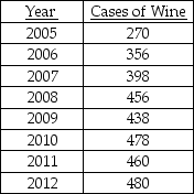-Referring to Table 16-1,set up a scatter diagram (i.e.,a time-series plot)with year on the horizontal X-axis.

TABLE 16-14 A contractor developed a multiplicative time-series model to forecast the number of contracts in future quarters,using quarterly data on number of contracts during the 3-year period from 2010 to 2012.The following is the resulting regression equation: ln = 3.37 + 0.117 X - 0.083 Q₁ + 1.28 Q₂ + 0.617 Q₃ where is the estimated number of contracts in a quarter X is the coded quarterly value with X = 0 in the first quarter of 2010 Q₁ is a dummy variable equal to 1 in the first quarter of a year and 0 otherwise Q₂ is a dummy variable equal to 1 in the second quarter of a year and 0 otherwise Q₃ is a dummy variable equal to 1 in the third quarter of a year and 0 otherwise -Referring to Table 16-14,using the regression equation,which of the following values is the best forecast for the number of contracts in the third quarter of 2013?

TABLE 16-7 The executive vice-president of a drug manufacturing firm believes that the demand for the firm's most popular drug has been evidencing an exponential trend since 1999.She uses Microsoft Excel to obtain the partial output below.The dependent variable is the log base 10 of the demand for the drug,while the independent variable is years,where 1999 is coded as 0,2000 is coded as 1,etc. SUMMARY OUTPUT Regression Statistics Multiple R 0.996 R Square 0.992 Adjusted R Square 0.991 Standard Error 0.02831 Observations 12 Coefficients Intercept 1.44 Coded Year 0.068 -Referring to Table 16-7,the forecast for the demand in 2013 is ________.

TABLE 16-3 The following table contains the number of complaints received in a department store for the first 6 months of last year. 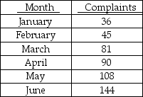-Referring to Table 16-3,if a three-month moving average is used to smooth this series,how many values would it have?

TABLE 16-13 Given below is the monthly time-series data for U.S.retail sales of building materials over a specific year. 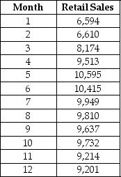The results of the linear trend,quadratic trend,exponential trend,first-order autoregressive,second-order autoregressive and third-order autoregressive model are presented below in which the coded month for the 1^st month is 0: Linear trend model: 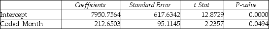Quadratic trend model: 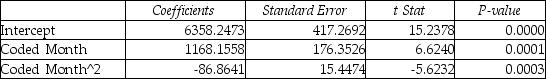Exponential trend model: First-order autoregressive: 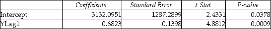Second-order autoregressive: 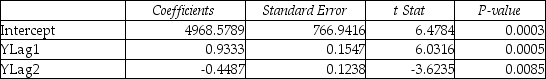Third-order autoregressive: 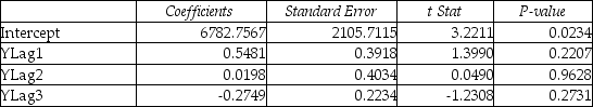Below is the residual plot of the various models: 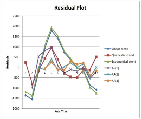-Referring to Table 16-13,construct a scatter plot (i.e.,a time-series plot)with month on the horizontal X-axis.

TABLE 16-11 The manager of a health club has recorded mean attendance in newly introduced step classes over the last 15 months: 32.1,39.5,40.3,46.0,65.2,73.1,83.7,106.8,118.0,133.1,163.3,182.8,205.6,249.1,and 263.5.She then used Microsoft Excel to obtain the following partial output for both a first- and second-order autoregressive model. SUMMARY OUTPUT - 2nd Order Model Regression Statistics Multiple R 0.993 R Square 0.987 Adjusted R Square 0.985 Standard Error 9.276 Observations 15 Coefficients Intercept 5.86 X Variable 1 0.37 X Variable 2 0.85 SUMMARY OUTPUT - 1st Order Model Regression Statistics Multiple R 0.993 R Square 0.987 Adjusted R Square 0.985 Standard Error 9.150 Observations 15 Coefficients Intercept 5.66 X Variable 1 1.10 -Referring to Table 16-11,using the second-order model,the forecast of mean attendance for month 17 is ________.

TABLE 16-13 Given below is the monthly time-series data for U.S.retail sales of building materials over a specific year. The results of the linear trend,quadratic trend,exponential trend,first-order autoregressive,second-order autoregressive and third-order autoregressive model are presented below in which the coded month for the 1^st month is 0: Linear trend model: Quadratic trend model: Exponential trend model: First-order autoregressive: Second-order autoregressive: Third-order autoregressive: Below is the residual plot of the various models: -Referring to Table 16-13,what is your forecast for the 13^th month using the quadratic-trend model?

TABLE 16-4 The number of cases of merlot wine sold by a Paso Robles winery in an 8-year period follows. 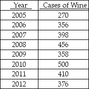-Referring to Table 16-4,exponential smoothing with a weight or smoothing constant of 0.4 will be used to smooth the wine sales.The value of E₅,the smoothed value for 2009 is ________.

TABLE 16-14 A contractor developed a multiplicative time-series model to forecast the number of contracts in future quarters,using quarterly data on number of contracts during the 3-year period from 2010 to 2012.The following is the resulting regression equation: ln = 3.37 + 0.117 X - 0.083 Q₁ + 1.28 Q₂ + 0.617 Q₃ where is the estimated number of contracts in a quarter X is the coded quarterly value with X = 0 in the first quarter of 2010 Q₁ is a dummy variable equal to 1 in the first quarter of a year and 0 otherwise Q₂ is a dummy variable equal to 1 in the second quarter of a year and 0 otherwise Q₃ is a dummy variable equal to 1 in the third quarter of a year and 0 otherwise -Referring to Table 16-14,the best interpretation of the coefficient of X (0.117)in the regression equation is

True or False: A least squares linear trend line is just a simple regression line with the years recorded.

TABLE 16-4 The number of cases of merlot wine sold by a Paso Robles winery in an 8-year period follows. -Referring to Table 16-4,exponentially smooth the wine sales with a weight or smoothing constant of 0.2.

TABLE 16-2 The monthly advertising expenditures of a department store chain (in $1,000,000s)were collected over the last decade.The last 14 months of this time series follows: 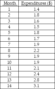-Referring to Table 16-2,set up a scatter plot (i.e.,time-series plot)with months on the horizontal X-axis.

Which of the following is not an advantage of exponential smoothing?

TABLE 16-14 A contractor developed a multiplicative time-series model to forecast the number of contracts in future quarters,using quarterly data on number of contracts during the 3-year period from 2010 to 2012.The following is the resulting regression equation: ln = 3.37 + 0.117 X - 0.083 Q₁ + 1.28 Q₂ + 0.617 Q₃ where is the estimated number of contracts in a quarter X is the coded quarterly value with X = 0 in the first quarter of 2010 Q₁ is a dummy variable equal to 1 in the first quarter of a year and 0 otherwise Q₂ is a dummy variable equal to 1 in the second quarter of a year and 0 otherwise Q₃ is a dummy variable equal to 1 in the third quarter of a year and 0 otherwise -Referring to Table 16-14,to obtain a forecast for the fourth quarter of 2013 using the model,which of the following sets of values should be used in the regression equation?

TABLE 16-12 A local store developed a multiplicative time-series model to forecast its revenues in future quarters,using quarterly data on its revenues during the 5-year period from 2008 to 2012.The following is the resulting regression equation: log₁₀ = 6.102 + 0.012 X - 0.129 Q₁ - 0.054 Q₂ + 0.098 Q₃ where is the estimated number of contracts in a quarter X is the coded quarterly value with X = 0 in the first quarter of 2008 Q₁ is a dummy variable equal to 1 in the first quarter of a year and 0 otherwise Q₂ is a dummy variable equal to 1 in the second quarter of a year and 0 otherwise is a dummy variable equal to 1 in the third quarter of a year and 0 otherwise -Referring to Table 16-12,to obtain a forecast for the third quarter of 2013 using the model,which of the following sets of values should be used in the regression equation?

TABLE 16-9 Given below are EXCEL outputs for various estimated autoregressive models for a company's real operating revenues (in billions of dollars)from 1989 to 2012.From the data,you also know that the real operating revenues for 2010,2011,and 2012 are 11.7909,11.7757 and 11.5537,respectively. First-Order Autoregressive Model: 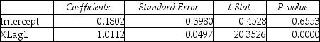Second-Order Autoregressive Model: 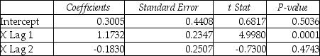Third-Order Autoregressive Model: 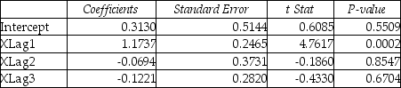-Referring to Table 16-9,if one decides to use the Third-Order Autoregressive model,what will the predicted real operating revenue for the company be in 2013?

TABLE 16-12 A local store developed a multiplicative time-series model to forecast its revenues in future quarters,using quarterly data on its revenues during the 5-year period from 2008 to 2012.The following is the resulting regression equation: log₁₀ = 6.102 + 0.012 X - 0.129 Q₁ - 0.054 Q₂ + 0.098 Q₃ where is the estimated number of contracts in a quarter X is the coded quarterly value with X = 0 in the first quarter of 2008 Q₁ is a dummy variable equal to 1 in the first quarter of a year and 0 otherwise Q₂ is a dummy variable equal to 1 in the second quarter of a year and 0 otherwise is a dummy variable equal to 1 in the third quarter of a year and 0 otherwise -Referring to Table 16-12,using the regression equation,what is the forecast for the revenues in the first quarter of 2015?

TABLE 16-13 Given below is the monthly time-series data for U.S.retail sales of building materials over a specific year. The results of the linear trend,quadratic trend,exponential trend,first-order autoregressive,second-order autoregressive and third-order autoregressive model are presented below in which the coded month for the 1^st month is 0: Linear trend model: Quadratic trend model: Exponential trend model: First-order autoregressive: Second-order autoregressive: Third-order autoregressive: Below is the residual plot of the various models: -Referring to Table 16-13,what is your estimated annual compound growth rate using the exponential-trend model?