Exam 15: Multiple Regression Model Building

An independent variable X_j is considered highly correlated with the other independent variables if

True or False: Collinearity is present if the dependent variable is linearly related to one of the explanatory variables.

TABLE 15-4 The superintendent of a school district wanted to predict the percentage of students passing a sixth-grade proficiency test.She obtained the data on percentage of students passing the proficiency test (% Passing),daily mean of the percentage of students attending class (% Attendance),mean teacher salary in dollars (Salaries),and instructional spending per pupil in dollars (Spending)of 47 schools in the state. Let Y = % Passing as the dependent variable,X₁ = % Attendance,X₂ = Salaries and X₃ = Spending. The coefficient of multiple determination ( )of each of the 3 predictors with all the other remaining predictors are,respectively,0.0338,0.4669,and 0.4743. The output from the best-subset regressions is given below: 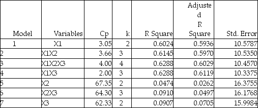Following is the residual plot for % Attendance: 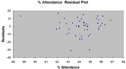Following is the output of several multiple regression models: Model (I): 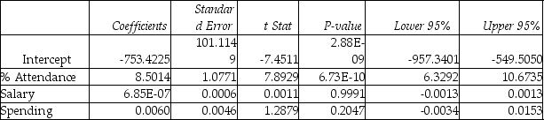Model (II): 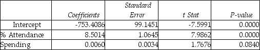Model (III): 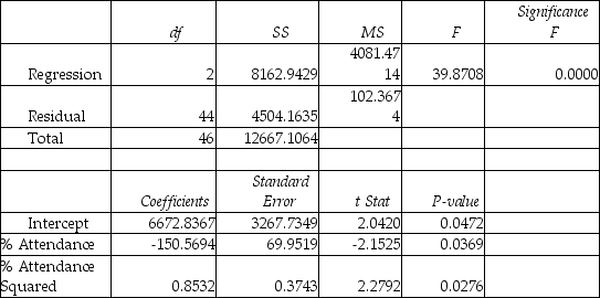-True or False: Referring to Table 15-4,the null hypothesis should be rejected when testing whether the quadratic effect of daily average of the percentage of students attending class on percentage of students passing the proficiency test is significant at a 5% level of significance.

TABLE 15-6 Given below are results from the regression analysis on 40 observations where the dependent variable is the number of weeks a worker is unemployed due to a layoff (Y)and the independent variables are the age of the worker (X₁),the number of years of education received (X₂),the number of years at the previous job (X₃),a dummy variable for marital status (X₄: 1 = married,0 = otherwise),a dummy variable for head of household (X₅: 1 = yes,0 = no)and a dummy variable for management position (X₆: 1 = yes,0 = no). The coefficient of multiple determination ( )for the regression model using each of the 6 variables X_j as the dependent variable and all other X variables as independent variables are,respectively,0.2628,0.1240,0.2404,0.3510,0.3342 and 0.0993. The partial results from best-subset regression are given below: 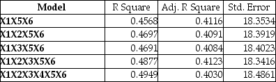-True or False: Referring to Table 15-6,the variable X₁ should be dropped to remove collinearity.

TABLE 15-6 Given below are results from the regression analysis on 40 observations where the dependent variable is the number of weeks a worker is unemployed due to a layoff (Y)and the independent variables are the age of the worker (X₁),the number of years of education received (X₂),the number of years at the previous job (X₃),a dummy variable for marital status (X₄: 1 = married,0 = otherwise),a dummy variable for head of household (X₅: 1 = yes,0 = no)and a dummy variable for management position (X₆: 1 = yes,0 = no). The coefficient of multiple determination ( )for the regression model using each of the 6 variables X_j as the dependent variable and all other X variables as independent variables are,respectively,0.2628,0.1240,0.2404,0.3510,0.3342 and 0.0993. The partial results from best-subset regression are given below: -True or False: Referring to Table 15-6,the variable X₂ should be dropped to remove collinearity.

TABLE 15-6 Given below are results from the regression analysis on 40 observations where the dependent variable is the number of weeks a worker is unemployed due to a layoff (Y)and the independent variables are the age of the worker (X₁),the number of years of education received (X₂),the number of years at the previous job (X₃),a dummy variable for marital status (X₄: 1 = married,0 = otherwise),a dummy variable for head of household (X₅: 1 = yes,0 = no)and a dummy variable for management position (X₆: 1 = yes,0 = no). The coefficient of multiple determination ( )for the regression model using each of the 6 variables X_j as the dependent variable and all other X variables as independent variables are,respectively,0.2628,0.1240,0.2404,0.3510,0.3342 and 0.0993. The partial results from best-subset regression are given below: -True or False: Referring to Table 15-6,the variable X₅ should be dropped to remove collinearity.

A microeconomist wants to determine how corporate sales are influenced by capital and wage spending by companies.She proceeds to randomly select 26 large corporations and record information in millions of dollars.A statistical analyst discovers that capital spending by corporations has a significant inverse relationship with wage spending.What should the microeconomist who developed this multiple regression model be particularly concerned with?

True or False: Referring to Table 15-3,suppose the chemist decides to use a t test to determine if there is a significant difference between a linear model and a curvilinear model that includes a linear term.If she used a level of significance of 0.01,she would decide that the linear model is sufficient.

The C_p statistic is used

TABLE 15-6 Given below are results from the regression analysis on 40 observations where the dependent variable is the number of weeks a worker is unemployed due to a layoff (Y)and the independent variables are the age of the worker (X₁),the number of years of education received (X₂),the number of years at the previous job (X₃),a dummy variable for marital status (X₄: 1 = married,0 = otherwise),a dummy variable for head of household (X₅: 1 = yes,0 = no)and a dummy variable for management position (X₆: 1 = yes,0 = no). The coefficient of multiple determination ( )for the regression model using each of the 6 variables X_j as the dependent variable and all other X variables as independent variables are,respectively,0.2628,0.1240,0.2404,0.3510,0.3342 and 0.0993. The partial results from best-subset regression are given below: -True or False: Referring to Table 15-6,the model that includes X₁,X₂,X₃,X₅ and X₆ should be among the appropriate models using the Mallow's C_p statistic.

TABLE 15-6 Given below are results from the regression analysis on 40 observations where the dependent variable is the number of weeks a worker is unemployed due to a layoff (Y)and the independent variables are the age of the worker (X₁),the number of years of education received (X₂),the number of years at the previous job (X₃),a dummy variable for marital status (X₄: 1 = married,0 = otherwise),a dummy variable for head of household (X₅: 1 = yes,0 = no)and a dummy variable for management position (X₆: 1 = yes,0 = no). The coefficient of multiple determination ( )for the regression model using each of the 6 variables X_j as the dependent variable and all other X variables as independent variables are,respectively,0.2628,0.1240,0.2404,0.3510,0.3342 and 0.0993. The partial results from best-subset regression are given below: -True or False: Referring to Table 15-6,the model that includes X₁,X₂,X₅ and X₆ should be among the appropriate models using the Mallow's C_p statistic.

True or False: One of the consequences of collinearity in multiple regression is inflated standard errors in some or all of the estimated slope coefficients.

TABLE 15-6 Given below are results from the regression analysis on 40 observations where the dependent variable is the number of weeks a worker is unemployed due to a layoff (Y)and the independent variables are the age of the worker (X₁),the number of years of education received (X₂),the number of years at the previous job (X₃),a dummy variable for marital status (X₄: 1 = married,0 = otherwise),a dummy variable for head of household (X₅: 1 = yes,0 = no)and a dummy variable for management position (X₆: 1 = yes,0 = no). The coefficient of multiple determination ( )for the regression model using each of the 6 variables X_j as the dependent variable and all other X variables as independent variables are,respectively,0.2628,0.1240,0.2404,0.3510,0.3342 and 0.0993. The partial results from best-subset regression are given below: -True or False: Referring to Table 15-6,the model that includes all the six independent variables should be among the appropriate models using the Mallow's C_p statistic.

TABLE 15-5 What are the factors that determine the acceleration time (in sec.)from 0 to 60 miles per hour of a car? Data on the following variables for 171 different vehicle models were collected: Accel Time: Acceleration time in sec. Cargo Vol: Cargo volume in cu.ft. HP: Horsepower MPG: Miles per gallon SUV: 1 if the vehicle model is an SUV with Coupe as the base when SUV and Sedan are both 0 Sedan: 1 if the vehicle model is a sedan with Coupe as the base when SUV and Sedan are both 0 The coefficient of multiple determination ( )for the regression model using each of the 5 variables X_j as the dependent variable and all other X variables as independent variables are,respectively,0.7461,0.5676,0.6764,0.8582,0.6632. -Referring to Table 15-5,what is the value of the variance inflationary factor of Cargo Vol?

TABLE 15-4 The superintendent of a school district wanted to predict the percentage of students passing a sixth-grade proficiency test.She obtained the data on percentage of students passing the proficiency test (% Passing),daily mean of the percentage of students attending class (% Attendance),mean teacher salary in dollars (Salaries),and instructional spending per pupil in dollars (Spending)of 47 schools in the state. Let Y = % Passing as the dependent variable,X₁ = % Attendance,X₂ = Salaries and X₃ = Spending. The coefficient of multiple determination ( )of each of the 3 predictors with all the other remaining predictors are,respectively,0.0338,0.4669,and 0.4743. The output from the best-subset regressions is given below: Following is the residual plot for % Attendance: Following is the output of several multiple regression models: Model (I): Model (II): Model (III): -Referring to Table 15-4,the better model using a 5% level of significance derived from the "best" model above is

True or False: In data mining where huge data sets are being explored to discover relationships among a large number of variables,the best-subsets approach is more practical than the stepwise regression approach.

True or False: Using the C_p statistic in model building,all models with C_p ≤ (k + 1)are equally good.

TABLE 15-4 The superintendent of a school district wanted to predict the percentage of students passing a sixth-grade proficiency test.She obtained the data on percentage of students passing the proficiency test (% Passing),daily mean of the percentage of students attending class (% Attendance),mean teacher salary in dollars (Salaries),and instructional spending per pupil in dollars (Spending)of 47 schools in the state. Let Y = % Passing as the dependent variable,X₁ = % Attendance,X₂ = Salaries and X₃ = Spending. The coefficient of multiple determination ( )of each of the 3 predictors with all the other remaining predictors are,respectively,0.0338,0.4669,and 0.4743. The output from the best-subset regressions is given below: Following is the residual plot for % Attendance: Following is the output of several multiple regression models: Model (I): Model (II): Model (III): -Referring to Table 15-4,which of the following models should be taken into consideration using the Mallows' C_p statistic?

True or False: Referring to Table 15-3,suppose the chemist decides to use an F test to determine if there is a significant curvilinear relationship between time and dose.If she chooses to use a level of significance of 0.01 she would decide that there is a significant curvilinear relationship.

True or False: Referring to Table 15-3,suppose the chemist decides to use a t test to determine if there is a significant difference between a linear model and a curvilinear model that includes a linear term.If she used a level of significance of 0.05,she would decide that the linear model is sufficient.