Exam 15: Multiple Regression Model Building

TABLE 15-5 What are the factors that determine the acceleration time (in sec.) from 0 to 60 miles per hour of a car? Data on the following variables for 171 different vehicle models were collected: Accel Time: Acceleration time in sec. Cargo Vol: Cargo volume in cu. ft. 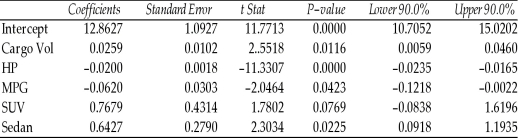HP: Horsepower MPG: Miles per gallon SUV: 1 if the vehicle model is an SUV with Coupe as the base when SUV and Sedan are both 0 Sedan: 1 if the vehicle model is a sedan with Coupe as the base when SUV and Sedan are both 0 The regression results using acceleration time as the dependent variable and the remaining variables as the independent variables are presented below. 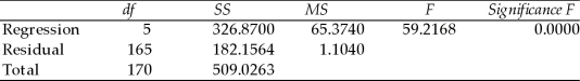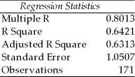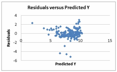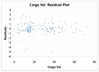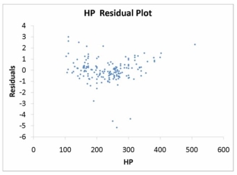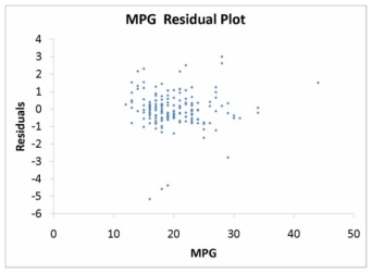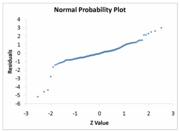ANOVA The various residual plots are as shown below. The coefficient of partial determination ( 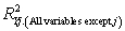) of each of the 5 predictors are, respectively, 0.0380, 0.4376, 0.0248, 0.0188, and 0.0312. The coefficient of multiple determination for the regression model using each of the 5 variables as the dependent variable and all other X variables as independent variables ( ) are, respectively, 0.7461, 0.5676, 0.6764, 0.8582, 0.6632. -Referring to Table 15-5, ________ of the variation in Accel Time can be explained by MPG while controlling for the other independent variables.

TABLE 15-5 What are the factors that determine the acceleration time (in sec.) from 0 to 60 miles per hour of a car? Data on the following variables for 171 different vehicle models were collected: Accel Time: Acceleration time in sec. Cargo Vol: Cargo volume in cu. ft. HP: Horsepower MPG: Miles per gallon SUV: 1 if the vehicle model is an SUV with Coupe as the base when SUV and Sedan are both 0 Sedan: 1 if the vehicle model is a sedan with Coupe as the base when SUV and Sedan are both 0 The regression results using acceleration time as the dependent variable and the remaining variables as the independent variables are presented below. ANOVA The various residual plots are as shown below. The coefficient of partial determination ( ) of each of the 5 predictors are, respectively, 0.0380, 0.4376, 0.0248, 0.0188, and 0.0312. The coefficient of multiple determination for the regression model using each of the 5 variables as the dependent variable and all other X variables as independent variables ( ) are, respectively, 0.7461, 0.5676, 0.6764, 0.8582, 0.6632. -Referring to Table 15-5, ________ of the variation in Accel Time can be explained by the five independent variables.

The logarithm transformation can be used

TABLE 15-2 In Hawaii, condemnation proceedings are under way to enable private citizens to own the property that their homes are built on. Until recently, only estates were permitted to own land, and homeowners leased the land from the estate. In order to comply with the new law, a large Hawaiian estate wants to use regression analysis to estimate the fair market value of the land. The following model was fit to data collected for n = 20 properties, 10 of which are located near a cove. Using the data collected for the 20 properties, the following partial output obtained from Microsoft Excel is shown: SUMMARY OUTPUT Regression Statistics ANOVA -Referring to Table 15-2, given a quadratic relationship between sale price (Y) and property size (X₁), what null hypothesis would you test to determine whether the curves differ from cove and non-cove properties?

TABLE 15-5 What are the factors that determine the acceleration time (in sec.) from 0 to 60 miles per hour of a car? Data on the following variables for 171 different vehicle models were collected: Accel Time: Acceleration time in sec. Cargo Vol: Cargo volume in cu. ft. HP: Horsepower MPG: Miles per gallon SUV: 1 if the vehicle model is an SUV with Coupe as the base when SUV and Sedan are both 0 Sedan: 1 if the vehicle model is a sedan with Coupe as the base when SUV and Sedan are both 0 The regression results using acceleration time as the dependent variable and the remaining variables as the independent variables are presented below. ANOVA The various residual plots are as shown below. The coefficient of partial determination ( ) of each of the 5 predictors are, respectively, 0.0380, 0.4376, 0.0248, 0.0188, and 0.0312. The coefficient of multiple determination for the regression model using each of the 5 variables as the dependent variable and all other X variables as independent variables ( ) are, respectively, 0.7461, 0.5676, 0.6764, 0.8582, 0.6632. -Referring to Table 15-5, the 0 to 60 miles per hour acceleration time of a sedan is predicted to be 0.6427 seconds higher than that of an SUV.

So that we can fit curves as well as lines by regression, we often use mathematical manipulations for converting one variable into a different form. These manipulations are called dummy variables.

TABLE 15-3 A chemist employed by a pharmaceutical firm has developed a muscle relaxant. She took a sample of 14 people suffering from extreme muscle constriction. She gave each a vial containing a dose (X) of the drug and recorded the time to relief (Y) measured in seconds for each. She fit a "centered" curvilinear model to this data. The results obtained by Microsoft Excel follow, where the dose (X) given has been "centered." SUMMARY OUTPUT Regression Statistics ANOVA -Referring to Table 15-3, suppose the chemist decides to use a t test to determine if there is a significant difference between a curvilinear model without a linear term and a curvilinear model that includes a linear term. The value of the test statistic is ________.

Which of the following is used to find a "best" model?

The Variance Inflationary Factor (VIF) measures the

As a project for his business statistics class, a student examined the factors that determined parking meter rates throughout the campus area. Data were collected for the price per hour of parking, blocks to the quadrangle, and one of the three jurisdictions: on campus, in downtown and off campus, or outside of downtown and off campus. The population regression model hypothesized is Y_i = α + β₀ + β₁X_1i + β₂X_2i + β₃X_3i + ε Where Y is the meter price X₁ is the number of blocks to the quad X₂ is a dummy variable that takes the value 1 if the meter is located in downtown and off campus and the value 0 otherwise X₃ is a dummy variable that takes the value 1 if the meter is located outside of downtown and off campus, and the value 0 otherwise Suppose that whether the meter is located on campus is an important explanatory factor. Why should the variable that depicts this attribute not be included in the model?

TABLE 15-3 A chemist employed by a pharmaceutical firm has developed a muscle relaxant. She took a sample of 14 people suffering from extreme muscle constriction. She gave each a vial containing a dose (X) of the drug and recorded the time to relief (Y) measured in seconds for each. She fit a "centered" curvilinear model to this data. The results obtained by Microsoft Excel follow, where the dose (X) given has been "centered." SUMMARY OUTPUT Regression Statistics ANOVA -Referring to Table 15-3, suppose the chemist decides to use a t test to determine if there is a significant difference between a curvilinear model without a linear term and a curvilinear model that includes a linear term. Using a level of significance of 0.05, she would decide that the curvilinear model should include a linear term.

The parameter estimates are biased when collinearity is present in a multiple regression equation.

TABLE 15-3 A chemist employed by a pharmaceutical firm has developed a muscle relaxant. She took a sample of 14 people suffering from extreme muscle constriction. She gave each a vial containing a dose (X) of the drug and recorded the time to relief (Y) measured in seconds for each. She fit a "centered" curvilinear model to this data. The results obtained by Microsoft Excel follow, where the dose (X) given has been "centered." SUMMARY OUTPUT Regression Statistics ANOVA -Referring to Table 15-3, suppose the chemist decides to use an F test to determine if there is a significant curvilinear relationship between time and dose. If she chooses to use a level of significance of 0.01 she would decide that there is a significant curvilinear relationship.

TABLE 15-4 The superintendent of a school district wanted to predict the percentage of students passing a sixth-grade proficiency test. She obtained the data on percentage of students passing the proficiency test (% Passing), daily average of the percentage of students attending class (% Attendance), average teacher salary in dollars (Salaries), and instructional spending per pupil in dollars (Spending) of 47 schools in the state. Let Y = % Passing as the dependent variable, X₁ = % Attendance, X₂ = Salaries and X₃ = Spending. The coefficient of multiple determination (R_j ²) of each of the 3 predictors with all the other remaining predictors are, respectively, 0.0338, 0.4669, and 0.4743. 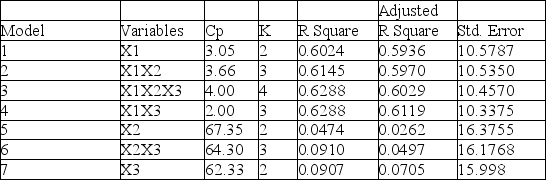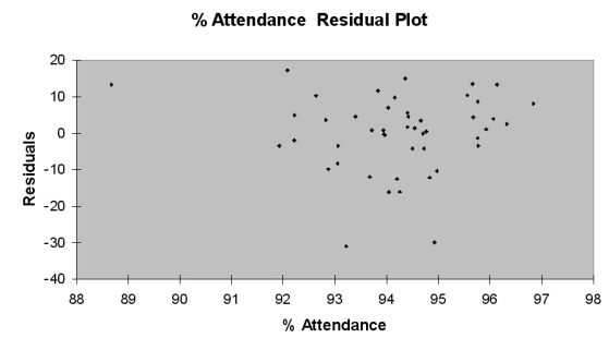The output from the best-subset regressions is given below: Following is the residual plot for % Attendance: Following is the output of several multiple regression models: Model (I): Model (II): Model (III): -Referring to Table 15-4, the "best" model chosen using the adjusted R-square statistic is

TABLE 15-4 The superintendent of a school district wanted to predict the percentage of students passing a sixth-grade proficiency test. She obtained the data on percentage of students passing the proficiency test (% Passing), daily average of the percentage of students attending class (% Attendance), average teacher salary in dollars (Salaries), and instructional spending per pupil in dollars (Spending) of 47 schools in the state. Let Y = % Passing as the dependent variable, X₁ = % Attendance, X₂ = Salaries and X₃ = Spending. The coefficient of multiple determination (R_j ²) of each of the 3 predictors with all the other remaining predictors are, respectively, 0.0338, 0.4669, and 0.4743. The output from the best-subset regressions is given below: Following is the residual plot for % Attendance: Following is the output of several multiple regression models: Model (I): Model (II): Model (III): -Referring to Table 15-4, there is reason to suspect collinearity between some pairs of predictors.

A regression diagnostic tool used to study the possible effects of collinearity is ________.

An independent variable X_j is considered highly correlated with the other independent variables if

TABLE 15-5 What are the factors that determine the acceleration time (in sec.) from 0 to 60 miles per hour of a car? Data on the following variables for 171 different vehicle models were collected: Accel Time: Acceleration time in sec. Cargo Vol: Cargo volume in cu. ft. HP: Horsepower MPG: Miles per gallon SUV: 1 if the vehicle model is an SUV with Coupe as the base when SUV and Sedan are both 0 Sedan: 1 if the vehicle model is a sedan with Coupe as the base when SUV and Sedan are both 0 The regression results using acceleration time as the dependent variable and the remaining variables as the independent variables are presented below. ANOVA The various residual plots are as shown below. The coefficient of partial determination ( ) of each of the 5 predictors are, respectively, 0.0380, 0.4376, 0.0248, 0.0188, and 0.0312. The coefficient of multiple determination for the regression model using each of the 5 variables as the dependent variable and all other X variables as independent variables ( ) are, respectively, 0.7461, 0.5676, 0.6764, 0.8582, 0.6632. -Referring to Table 15-5, which of the following assumptions is most likely violated based on the residual plot of the residuals versus predicted Y?

TABLE 15-4 The superintendent of a school district wanted to predict the percentage of students passing a sixth-grade proficiency test. She obtained the data on percentage of students passing the proficiency test (% Passing), daily average of the percentage of students attending class (% Attendance), average teacher salary in dollars (Salaries), and instructional spending per pupil in dollars (Spending) of 47 schools in the state. Let Y = % Passing as the dependent variable, X₁ = % Attendance, X₂ = Salaries and X₃ = Spending. The coefficient of multiple determination (R_j ²) of each of the 3 predictors with all the other remaining predictors are, respectively, 0.0338, 0.4669, and 0.4743. The output from the best-subset regressions is given below: Following is the residual plot for % Attendance: Following is the output of several multiple regression models: Model (I): Model (II): Model (III): -Referring to Table 15-4, what are, respectively, the values of the variance inflationary factor of the 3 predictors?

TABLE 15-5 What are the factors that determine the acceleration time (in sec.) from 0 to 60 miles per hour of a car? Data on the following variables for 171 different vehicle models were collected: Accel Time: Acceleration time in sec. Cargo Vol: Cargo volume in cu. ft. HP: Horsepower MPG: Miles per gallon SUV: 1 if the vehicle model is an SUV with Coupe as the base when SUV and Sedan are both 0 Sedan: 1 if the vehicle model is a sedan with Coupe as the base when SUV and Sedan are both 0 The regression results using acceleration time as the dependent variable and the remaining variables as the independent variables are presented below. ANOVA The various residual plots are as shown below. The coefficient of partial determination ( ) of each of the 5 predictors are, respectively, 0.0380, 0.4376, 0.0248, 0.0188, and 0.0312. The coefficient of multiple determination for the regression model using each of the 5 variables as the dependent variable and all other X variables as independent variables ( ) are, respectively, 0.7461, 0.5676, 0.6764, 0.8582, 0.6632. -Referring to Table 15-5, ________ of the variation in Accel Time can be explained by HP while controlling for the other independent variables.