Question 1

The OLS estimator

Accepted Answer

A) has the multivariate normal asymptotic distribution in large samples. 
B) is t-distributed. 
C) has the multivariate normal distribution regardless of the sample size. 
D) is F-distributed. 
A) has the multivariate normal asymptotic distribution in large samples. 
B) is t-distributed. 
C) has the multivariate normal distribution regardless of the sample size. 
D) is F-distributed. A

Question 2

Write the following four restrictions in the form $\boldsymbol { R } \boldsymbol { \beta } = \boldsymbol { r } ,$ where the hypotheses are to be tested simultaneously.
$\begin{array} { l } 
\beta _ { 3 } = 2 \beta _ { 5 } , \
\beta _ { 1 } + \beta _ { 2 } = 1 , \
\beta _ { 4 } = 0 , \
\beta _ { 2 } = - \beta _ { 6 } .
\end{array}$
Can you write the following restriction $\beta _ { 2 } = - \frac { \beta _ { 3 } } { \beta _ { 1 } }$ in the same format? Why not?

Accepted Answer

$\left( \begin{array} { c c c c c c c } 
0 & 0 & 0 & 1 & 0 & - 2 & 0 \
0 & 1 & 1 & 0 & 0 & 0 & 0 \
0 & 0 & 0 & 0 & 1 & 0 & 0 \
0 & 0 & 1 & 0 & 0 & 0 & 1
\end{array} \right) \left( \begin{array} { l } 
\beta _ { 0 } \
\beta _ { 1 } \
\beta _ { 2 } \
\beta _ { 3 } \
\beta _ { 4 } \
\beta _ { 5 } \
\beta _ { 6 }
\end{array} \right) = \left( \begin{array} { l } 
0 \
1 \
0 \
0
\end{array} \right)$
The restriction $\beta _ { 2 } = - \frac { \beta _ { 3 } } { \beta _ { 1 } }$ cannot be written in the same format because it is nonlinear.

Question 3

Write an essay on the difference between the OLS estimator and the GLS estimator.

Accepted Answer

Answers will vary by student, but some of the following points should be made.
The multiple regression model is $$Y _ { i } = \beta _ { 0 } + \beta _ { 1 } X _ { 1 i } + \beta _ { 2 } X _ { 2 i } + \cdots + \beta _ { k } X _ { k i } + u _ { i } , i = 1 , \ldots , n$$
which, in matrix form, can be written as $\boldsymbol { Y } = \boldsymbol { X } \boldsymbol { \beta } + \boldsymbol { U }$. The OLS estimator is derived by minimizing the squared prediction mistakes and results in the following formula: $\hat { \boldsymbol { \beta } } = \left( \boldsymbol { X } ^ { \prime } \boldsymbol { X } \right) ^ { - 1 } \boldsymbol { X } ^ { \prime } \boldsymbol { Y }$. There are two GLS estimators. The infeasible GLS estimator is $\hat { \boldsymbol { \beta } } ^ { G L S } = \left( \boldsymbol { X } ^ { \prime } \boldsymbol { \Omega } ^ { 1 }  \boldsymbol { X } \right) ^ { - 1 } \left( \boldsymbol { X } ^ { \prime } \boldsymbol { \Omega } ^ { 1 } \boldsymbol { Y } \right)$. Since $\Omega$ is typically unknown, the estimator cannot be calculated, and hence its name. However, a feasible GLS estimator can be calculated if $\Omega$ is a known function of a number of parameters which can be estimated. Once these parameters have been estimated, they can then be used to calculate $\hat { \Omega }$, the estimator of $\Omega$. The feasible GLS estimator is defined as $\hat { \boldsymbol { \beta } } ^ { G L S } = \left( \boldsymbol { X } ^ { \prime } \hat { \boldsymbol { \Omega } } ^ { - 1 } \boldsymbol { X } \right) ^ { - 1 } \left( \boldsymbol { X } ^ { \boldsymbol {} } \hat { \boldsymbol { \Omega } } ^ { - 1 } \boldsymbol { Y } \right)$. There are extended least squares assumptions.

Question 4

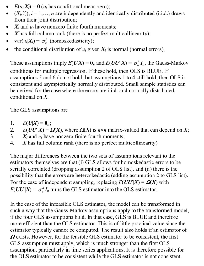
The multiple regression model can be written in matrix form as follows: a. $\boldsymbol { Y } = \boldsymbol { X } \boldsymbol { \beta }$.
b. $\boldsymbol { Y } = \boldsymbol { X } + \boldsymbol { U }$.
c. $\boldsymbol { Y } = \boldsymbol { \beta } \boldsymbol { X } + \boldsymbol { U }$.
d. $\boldsymbol { Y } = \boldsymbol { X } \boldsymbol { \beta } + \boldsymbol { U }$.

Accepted Answer

The answer of The multiple regression model can be written...

Question 5

The Gauss-Markov theorem for multiple regressions states that the OLS estimator

Accepted Answer

A) has the smallest variance possible for any linear estimator. 
B) is BLUE if the Gauss-Markov conditions for multiple regression hold. 
C) is identical to the maximum likelihood estimator. 
D) is the most commonly used estimator. 
A) has the smallest variance possible for any linear estimator. 
B) is BLUE if the Gauss-Markov conditions for multiple regression hold. 
C) is identical to the maximum likelihood estimator. 
D) is the most commonly used estimator.

Question 6

Assume that the data looks as follows: $$\boldsymbol { Y } = \left( \begin{array} { l } 
Y _ { 1 } \
Y _ { 2 } \
\vdots \
Y _ { n }
\end{array} \right) , \boldsymbol { U } = \left( \begin{array} { l } 
u _ { 1 } \
u _ { 2 } \
\vdots \
u _ { n }
\end{array} \right) , \boldsymbol { X } = \left( \begin{array} { c } 
X _ { 11 } \
X _ { 12 } \
\vdots \
X _ { 1 n }
\end{array} \right) \text {, and } \boldsymbol { \beta } = \left( \beta _ { 1 } \right)$$ Using the formula for the OLS estimator $\hat { \boldsymbol { \beta } } = \left( \boldsymbol { X } ^ { \prime } \boldsymbol { X } \right) ^ { - 1 } \boldsymbol { X } ^ { \prime } \boldsymbol { Y }$, derive the formula for $\widehat { \beta } _ { 1 }$, the only slope in this "regression through the origin."

Accepted Answer

The answer of Assume that the data looks as follows:...

Question 7

The presence of correlated error terms creates problems for inference based on OLS. These can be overcome by

Accepted Answer

A) using HAC standard errors. 
B) using heteroskedasticity-robust standard errors. 
C) reordering the observations until the correlation disappears. 
D) using homoskedasticity-only standard errors. 
A) using HAC standard errors. 
B) using heteroskedasticity-robust standard errors. 
C) reordering the observations until the correlation disappears. 
D) using homoskedasticity-only standard errors.

Question 8

Write the following three linear equations in matrix format $A x = b$, where $\boldsymbol { x }$ is a $3 \times 1$ vector containing $q , p$, and $y , \boldsymbol { A }$ is a $3 \times 3$ matrix of coefficients, and $\boldsymbol { b }$ is a $3 \times 1$ vector of constants. q = 5 +3 p - 2 y
q = 10 - p + 10 y
p = 6 y

Accepted Answer

The answer of Write the following three linear equations in...

Question 9

Given the following matrices $$\boldsymbol { A } = \left( \begin{array} { l l } 
a _ { 11 } & a _ { 12 } \
a _ { 21 } & a _ { 22 }
\end{array} \right) , \boldsymbol { B } = \left( \begin{array} { l l } 
b _ { 11 } & b _ { 12 } \
b _ { 21 } & b _ { 22 }
\end{array} \right) , \text { and } \boldsymbol { C } = \left( \begin{array} { l l l } 
c _ { 11 } & c _ { 12 } & c _ { 13 } \
c _ { 21 } & c _ { 22 } & c _ { 23 }
\end{array} \right)$$
show that $( \boldsymbol { A } + \boldsymbol { B } ) ^ { \prime } = \boldsymbol { A } ^ { \prime } + \boldsymbol { B } ^ { \prime }$ and $( \boldsymbol { A } \boldsymbol { C } ) ^ { \prime } = \boldsymbol { C } ^ { \prime } \boldsymbol { A } ^ { \prime }$.

Accepted Answer

The answer of Given the following matrices \[\boldsymbol { A...

Question 10

A joint hypothesis that is linear in the coefficients and imposes a number of restrictions can be written as a. $\left( \boldsymbol { X } ^ { \prime } \boldsymbol { X } \right) ^ { - 1 } \boldsymbol { X } ^ { \prime } \boldsymbol { Y }$.
b. $\boldsymbol { R } \boldsymbol { \beta } = \boldsymbol { r }$.
c. $\hat { \beta } - \beta$.
d. $\boldsymbol { R } \boldsymbol { \beta } = \mathbf { 0 }$.

Accepted Answer

The answer of A joint hypothesis that is linear in...

Question 11

The GLS estimator is defined as a.$\left(\boldsymbol{X}^{\prime} \boldsymbol{\Omega}^{1} \boldsymbol{X}\right)^{-1}\left(\boldsymbol{X}^{\prime} \Omega^{1} \boldsymbol{Y}\right)$ 
b. $\left( \boldsymbol { X } ^ { \prime } \boldsymbol { X } \right) ^ { - 1 } \boldsymbol { X } ^ { \prime } \boldsymbol { Y }$.
c. $A ^ { \prime } Y$.
d. $\left( \boldsymbol { X } ^ { \prime } \boldsymbol { X } \right) ^ { - 1 } \boldsymbol { X } ^ { \prime } \boldsymbol { U }$.

Accepted Answer

The answer of The GLS estimator is defined as a.\(\left(\boldsymbol{X}^{\prime}...

Question 12

In Chapter 10 of your textbook, panel data estimation was introduced.Panel data consist
of observations on the same n entities at two or more time periods T.For two variables,
you have $$\left( X _ { i t } , Y _ { i t } \right) , i = 1 , \ldots , n \text { and } t = 1 , \ldots , T$$ where n could be the U.S.states.The example in Chapter 10 used annual data from 1982
to 1988 for the fatality rate and beer taxes.Estimation by OLS, in essence, involved
"stacking" the data.
(a)What would the variance-covariance matrix of the errors look like in this case if you
allowed for homoskedasticity-only standard errors? What is its order? Use an example of
a linear regression with one regressor of 4 U.S.states and 3 time periods.

Accepted Answer

Answer @#IMG-DLM& @#IMG-DLM& (There is a subtle issue here f

Question 13

Using the model $\boldsymbol { Y } = \boldsymbol { X } \boldsymbol { \beta } + \boldsymbol { U }$ and the extended least squares assumptions, derive the OLS estimator  $\hat { \beta }$. Discuss the conditions under which $\boldsymbol { X } ^ { \prime } \boldsymbol { X }$ is invertible.

Accepted Answer

The answer of Using the model \(\boldsymbol { Y }...

Question 14

One of the properties of the OLS estimator is a. $\boldsymbol { X } \hat { \boldsymbol { \beta } } = \mathbf { 0 } _ { k + 1 }$.
b. that the coefficient vector $\hat { \beta }$has full rank.
c. $\boldsymbol { X } ^ { \prime } ( \boldsymbol { Y } - \boldsymbol { X } \hat { \boldsymbol { \beta } } ) = \mathbf { 0 } _ { k + 1 }$.
d. $\left( \boldsymbol { X } ^ { \prime } \boldsymbol { X } \right) ^ { - 1 } = \boldsymbol { X } ^ { \boldsymbol {} } \boldsymbol { Y }$

Accepted Answer

The answer of One of the properties of the OLS...

Question 15

The difference between the central limit theorems for a scalar and vector-valued random variables is

Accepted Answer

A) that n approaches infinity in the central limit theorem for scalars only. 
B) the conditions on the variances. 
C) that single random variables can have an expected value but vectors cannot. 
D) the homoskedasticity assumption in the former but not the latter. 
A) that n approaches infinity in the central limit theorem for scalars only. 
B) the conditions on the variances. 
C) that single random variables can have an expected value but vectors cannot. 
D) the homoskedasticity assumption in the former but not the latter.

Question 16

An estimator of $\beta$  is said to be linear if

Accepted Answer

A)  it can be estimated by least squares. 
B)  it is a linear function of $Y _ { 1 } , \ldots , Y _ { n }$ 
C)  there are homoskedasticity-only errors. 
D)  it is a linear function of $X _ { 1 } , \ldots , X _ { n }$ 
A)  it can be estimated by least squares. 
B)  it is a linear function of $Y _ { 1 } , \ldots , Y _ { n }$ 
C)  there are homoskedasticity-only errors. 
D)  it is a linear function of $X _ { 1 } , \ldots , X _ { n }$

Question 17

In the case when the errors are homoskedastic and normally distributed, conditional on X, then a. $\hat { \boldsymbol { \beta } }$ is distributed $N \left( \boldsymbol { \beta } , \Sigma _ { \hat { \beta } \mid X } \right)$, where $\Sigma _ { \hat { \beta } \mid X } = \sigma _ { u } ^ { 2 } \boldsymbol { I } _ { ( \mathrm { k } + 1 ) }$.
b. $\hat { \boldsymbol { \beta } }$ is distributed $\mathrm { N } \left( \boldsymbol { \beta } , \Sigma _ { \hat { \beta } } \right)$, where $\Sigma _ { \hat { \beta } } = \Sigma _ { \sqrt { n } ( \dot { \beta } - \beta ) } / n = \boldsymbol { Q } _ { X } ^ { - 1 } \Sigma _ { V } \boldsymbol { Q } _ { X } ^ { - 1 } / n$.
c. $\hat { \beta }$ is distributed $N \left( \boldsymbol { \beta } , \Sigma _ { \dot { \beta } \mid X } \right)$, where $\Sigma _ { \dot { \beta } \mid X } = \sigma _ { u } ^ { 2 } ( \boldsymbol { X } \boldsymbol { X } ) ^ { - 1 }$.
d. $\hat { U } = \boldsymbol { P } _ { \boldsymbol { X } } \boldsymbol { Y }$ where $\boldsymbol { P } _ { \boldsymbol { X } } = \boldsymbol { X } \left( \boldsymbol { X } ^ { \prime } \boldsymbol { X } \right) ^ { - 1 } \boldsymbol { X } ^ { \prime }$.

Accepted Answer

The answer of In the case when the errors are...

Question 18

Consider the multiple regression model from Chapter 5, where k = 2 and the assumptions
of the multiple regression model hold.
(a)Show what the X matrix and the $$\beta$$ vector would look like in this case.

Accepted Answer

The first order cond

Question 19

In order for a matrix A to have an inverse, its determinant cannot be zero.Derive the
determinant of the following matrices: $$A = \left( \begin{array} { c c } 
3 & 6 \
- 2 & 1
\end{array} \right)$$
$$B = \left( \begin{array} { c c c } 
1 & - 1 & 2 \
1 & 0 & 3 \
4 & 0 & 2
\end{array} \right)$$
$\boldsymbol { X } ^ { \prime } \boldsymbol { X }$ where $X = \left( \begin{array} { l l } 1 & 10 \end{array} \right)$

Accepted Answer

The answer of In order for a matrix A to...

Question 20

One implication of the extended least squares assumptions in the multiple regression model is that a. feasible GLS should be used for estimation.
b. $E ( \boldsymbol { U } \mid \boldsymbol { X } ) = \boldsymbol { I } _ { n }$.
c. $\boldsymbol { X } ^ { \prime } \boldsymbol { X }$ is singular.
d. the conditional distribution of $\boldsymbol { U }$ given $\boldsymbol { X }$ is $N \left( \mathbf { 0 } _ { n } , \sigma _ { u } ^ { 2 } \boldsymbol { I } _ { n } \right)$.

Accepted Answer

The answer of One implication of the extended least squares...

The OLS estimator

Write an essay on the difference between the OLS estimator and the GLS estimator.

The Gauss-Markov theorem for multiple regressions states that the OLS estimator

The presence of correlated error terms creates problems for inference based on OLS. These can be overcome by

Using the model $\boldsymbol { Y } = \boldsymbol { X } \boldsymbol { \beta } + \boldsymbol { U }$ and the extended least squares assumptions, derive the OLS estimator $\hat { \beta }$ . Discuss the conditions under which $\boldsymbol { X } ^ { \prime } \boldsymbol { X }$ is invertible.

The difference between the central limit theorems for a scalar and vector-valued random variables is

An estimator of $\beta$ is said to be linear if

Consider the multiple regression model from Chapter 5, where k = 2 and the assumptions of the multiple regression model hold. (a)Show what the X matrix and the $\beta$ vector would look like in this case.

Economic Questions and Data

Review of Probability

Review of Statistics

Linear Regression With One Regressor

Regression With a Single Regressor: Hypothesis Tests and Confidence Intervals

Linear Regression With Multiple Regressors

Hypothesis Tests and Confidence Intervals in Multiple Regression

Nonlinear Regression Functions

Assessing Studies Based on Multiple Regression

Regression With Panel Data

Regression With a Binary Dependent Variable

Instrumental Variables Regression

Experiments and Quasi-Experiments

Introduction to Time Series Regression and Forecasting

Estimation of Dynamic Causal Effects

Additional Topics in Time Series Regression

The Theory of Linear Regression With One Regressor

Filters

Exam 18: The Theory of Multiple Regression

The OLS estimator

Write an essay on the difference between the OLS estimator and the GLS estimator.

The Gauss-Markov theorem for multiple regressions states that the OLS estimator

The presence of correlated error terms creates problems for inference based on OLS. These can be overcome by

The difference between the central limit theorems for a scalar and vector-valued random variables is

An estimator of β\betaβ is said to be linear if

Consider the multiple regression model from Chapter 5, where k = 2 and the assumptions of the multiple regression model hold. (a)Show what the X matrix and the β\betaβ vector would look like in this case.

Economic Questions and Data

Review of Probability

Review of Statistics

Linear Regression With One Regressor

Regression With a Single Regressor: Hypothesis Tests and Confidence Intervals

Linear Regression With Multiple Regressors

Hypothesis Tests and Confidence Intervals in Multiple Regression

Nonlinear Regression Functions

Assessing Studies Based on Multiple Regression

Regression With Panel Data

Regression With a Binary Dependent Variable

Instrumental Variables Regression

Experiments and Quasi-Experiments

Introduction to Time Series Regression and Forecasting

Estimation of Dynamic Causal Effects

Additional Topics in Time Series Regression

The Theory of Linear Regression With One Regressor

Filters

An estimator of $\beta$ is said to be linear if

Consider the multiple regression model from Chapter 5, where k = 2 and the assumptions of the multiple regression model hold. (a)Show what the X matrix and the $\beta$ vector would look like in this case.