Attendance at sports events depends on various factors.Teams typically do not change ticket prices from game to game to attract more spectators to less attractive games. However, there are other marketing tools used, such as fireworks, free hats, etc., for this purpose.You work as a consultant for a sports team, the Los Angeles Dodgers, to help them forecast attendance, so that they can potentially devise strategies for price discrimination.After collecting data over two years for every one of the 162 home games of the 2000 and 2001 season, you run the following regression: \[\begin{array} { l } \widehat { \text { Attend } } = 15,005 + 201 \times \text { Temperat } + 465 \times \text { DodgNetWin } + 82 \times \text { OppNetWin } \\ + 9647 \times \text { DFSaSu } + 1328 \times \text { Drain } + 1609 \times \text { D } 150 m + 271 \times \text { DDiv } - 978 \times \text { D } 2001 ; \\ R ^ { 2 } = 0.416 , S E R = 6983 \end{array}\] where Attend is announced stadium attendance, Temperat it the average temperature on game day, DodgNetWin are the net wins of the Dodgers before the game (wins-losses), OppNetWin is the opposing team's net wins at the end of the previous season, and DFSaSu, Drain, D150m, Ddiv, and D2001 are binary variables, taking a value of 1 if the game was played on a weekend, it rained during that day, the opposing team was within a 150 mile radius, the opposing team plays in the same division as the Dodgers, and the game was played during 2001, respectively. (a)Interpret the regression results.Do the coefficients have the expected signs?

If there was a serious capacity constrai

The cost of attending your college has once again gone up.Although you have been told that education is investment in human capital, which carries a return of roughly 10% a year, you (and your parents)are not pleased.One of the administrators at your university/college does not make the situation better by telling you that you pay more because the reputation of your institution is better than that of others.To investigate this hypothesis, you collect data randomly for 100 national universities and liberal arts colleges from the 2000-2001 U.S.News and World Report annual rankings.Next you perform the following regression \[\begin{array} { l } \widehat { \text { Cost } } = 7,311.17 + 3,985.20 \times \text { Reputation } - 0.20 \times \text { Size } \\ + 8,406.79 \times \text { Dpriv } - 416.38 \times \text { Dlibart } - 2,376.51 \times \text { Dreligion } \\ R ^ { 2 } = 0.72 , \text { SER } = 3,773.35 \end{array}\] where Cost is Tuition, Fees, Room and Board in dollars, Reputation is the index used in U.S.News and World Report (based on a survey of university presidents and chief academic officers), which ranges from 1 ("marginal")to 5 ("distinguished"), Size is the number of undergraduate students, and Dpriv, Dlibart, and Dreligion are binary variables indicating whether the institution is private, a liberal arts college, and has a religious affiliation. (a)Interpret the results.Do the coefficients have the expected sign?

It is very possible that the university

Exam 6: Linear Regression With Multiple Regressors

You have collected data from Major League Baseball (MLB)to find the determinants of winning.You have a general idea that both good pitching and strong hitting are needed to do well.However, you do not know how much each of these contributes separately.To investigate this problem, you collect data for all MLB during 1999 season.Your strategy is to first regress the winning percentage on pitching quality ("Team ERA"), second to regress the same variable on some measure of hitting ("OPS - On-base Plus Slugging percentage"), and third to regress the winning percentage on both. Summary of the Distribution of Winning Percentage, On Base plus Slugging percentage, and Team Earned Run Average for MLB in 1999 $You have collected data from Major League Baseball (MLB)to find the determinants of winning.You have a general idea that both good pitching and strong hitting are needed to do well.However, you do not know how much each of these contributes separately.To investigate this problem, you collect data for all MLB during 1999 season.Your strategy is to first regress the winning percentage on pitching quality (Team ERA), second to regress the same variable on some measure of hitting (OPS - On-base Plus Slugging percentage), and third to regress the winning percentage on both. Summary of the Distribution of Winning Percentage, On Base plus Slugging percentage, and Team Earned Run Average for MLB in 1999 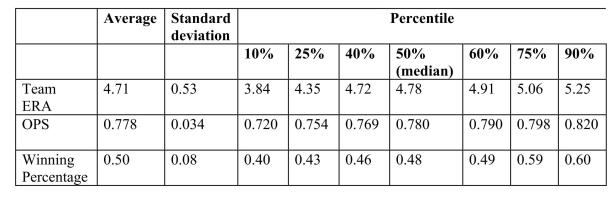The results are as follows: \widehat { \text { Winpct } } = 0.94 - 0.100 \times \text { teamera } , \quad R ^ { 2 } = 0.49 , S E R = 0.06 \text {. } \widehat { \text { Winpct } } = - 0.68 + 1.513 \times ops, R ^ { 2 } = 0.45 , SER = 0.06 . \widehat { \text { Winpct } } = - 0.19 - 0.099 \times \text { teamera } + 1.490 \times \text { ops } , R ^ { 2 } = 0.92 , S E R = 0.02 \text {. } (a)Interpret the multiple regression.What is the effect of a one point increase in team ERA? Given that the Atlanta Braves had the most wins that year, wining 103 games out of 162, do you find this effect important? Next analyze the importance and statistical significance for the OPS coefficient.(The Minnesota Twins had the minimum OPS of 0.712, while the Texas Rangers had the maximum with 0.840.)Since the intercept is negative, and since winning percentages must lie between zero and one, should you rerun the regression through the origin?$ The results are as follows: $\widehat { \text { Winpct } } = 0.94 - 0.100 \times \text { teamera } , \quad R ^ { 2 } = 0.49 , S E R = 0.06 \text {. }$ $\widehat { \text { Winpct } } = - 0.68 + 1.513 \times$ ops, $R ^ { 2 } = 0.45$ , SER $= 0.06$ . $\widehat { \text { Winpct } } = - 0.19 - 0.099 \times \text { teamera } + 1.490 \times \text { ops } , R ^ { 2 } = 0.92 , S E R = 0.02 \text {. }$ (a)Interpret the multiple regression.What is the effect of a one point increase in team ERA? Given that the Atlanta Braves had the most wins that year, wining 103 games out of 162, do you find this effect important? Next analyze the importance and statistical significance for the OPS coefficient.(The Minnesota Twins had the minimum OPS of 0.712, while the Texas Rangers had the maximum with 0.840.)Since the intercept is negative, and since winning percentages must lie between zero and one, should you rerun the regression through the origin?

Free

(Essay)

4.9/5

(37)

Question 1

Correct Answer:

Verified

The quality of the management and coaching comes to mind, although both
may be reflected in the performance statistics, as are salaries.There are other
aspects of baseball performance that are missing, such as the fielding percentage
of the team.

You have to worry about perfect multicollinearity in the multiple regression model because

Free

(Multiple Choice)

4.7/5

(38)

Question 2

Correct Answer:

Verified

Your econometrics textbook stated that there will be omitted variable bias in the OLS estimator unless the included regressor, X, is uncorrelated with the omitted variable or the omitted variable is not a determinant of the dependent variable, Y.Give an intuitive explanation for these two conditions.

Free

(Essay)

4.7/5

(45)

Question 3

Correct Answer:

Verified

The regression coefficient is the partial derivative of Y with respect to the
corresponding X.The meaning of the partial derivative is the effect of a change
in X on Y, holding all the other variables constant.This is identical to a
controlled laboratory experiment where only one variable is changed at a time,
while all the other variables are held constant.In real life, of course, you cannot
change one variable and keep all others, including the omitted variables,
constant.
Now consider the case of X changing.If it is correlated with the omitted
variable and if that variable is a determinant of Y, then Y will change further as a
result of X changing.This will cause the "controlled experiment" measure to
over or understate the effect that X has on Y, depending on the relationship
between X and the omitted variable.If X is not correlated with the omitted
variable, then changing X will not have this further indirect effect on Y, so that
the pure relationship between X and Y can be measured because it is "as if" the
omitted variable were held constant.This has important practical implications if
data is hard to obtain for an omitted variable while it can be argued that the
variable of interest is not much correlated with the omitted variable.
Y will change when a relevant omitted variable will change, and hence the pure
effect of X on Y cannot be observed.In the laboratory, Y would change for
reasons unrelated to the change in X.However, if the omitted variable is not a
determinant of Y, then a change in it will have no effect on the pure relationship
between X and Y.
Consider the accompanying graph of the determinants of Y, where X is the
included variable and Z the omitted variable. 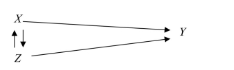Then the effect of X on Y can be measured properly as long as the arrow from Z
to Y does not exist, or as long as changes in X do not cause changes in Z, which
in return influence Y.

Attendance at sports events depends on various factors.Teams typically do not change ticket prices from game to game to attract more spectators to less attractive games. However, there are other marketing tools used, such as fireworks, free hats, etc., for this purpose.You work as a consultant for a sports team, the Los Angeles Dodgers, to help them forecast attendance, so that they can potentially devise strategies for price discrimination.After collecting data over two years for every one of the 162 home games of the 2000 and 2001 season, you run the following regression: =15,005+201\times Temperat +465\times DodgNetWin +82\times OppNetWin +9647\times DFSaSu +1328\times Drain +1609\times D 150m+271\times DDiv -978\times D 2001; =0.416,SER=6983 where Attend is announced stadium attendance, Temperat it the average temperature on game day, DodgNetWin are the net wins of the Dodgers before the game (wins-losses), OppNetWin is the opposing team's net wins at the end of the previous season, and DFSaSu, Drain, D150m, Ddiv, and D2001 are binary variables, taking a value of 1 if the game was played on a weekend, it rained during that day, the opposing team was within a 150 mile radius, the opposing team plays in the same division as the Dodgers, and the game was played during 2001, respectively. (a)Interpret the regression results.Do the coefficients have the expected signs?

(Essay)

4.9/5

(32)

Question 4

The population multiple regression model when there are two regressors, $X _ { 1 i } \text { and } X _ { 2 i }$ can be written as follows, with the exception of:

(Multiple Choice)

4.9/5

(33)

Question 5

In the multiple regression model with two regressors, the formula for the slope of the first explanatory variable is $\hat { \beta } _ { 1 } = \frac { \sum _ { i = 1 } ^ { n } y _ { i } x _ { 1 i } \sum _ { i = 1 } ^ { n } x _ { 2 i } ^ { 2 } - \sum _ { i = 1 } ^ { n } y _ { i } x _ { 2 i } \sum _ { i = 1 } ^ { n } x _ { 1 i } x _ { 2 i } } { \sum _ { i = 1 } ^ { n } x _ { 1 i } ^ { 2 } \sum _ { i = 1 } ^ { n } x _ { 2 i } ^ { 2 } - \left( \sum _ { i = 1 } ^ { n } x _ { 1 i } x _ { 2 i } \right) ^ { 2 } }$ (small letters refer to deviations from means as in $z _ { i } = Z _ { i } - \bar { Z }$ ). An alternative way to derive the OLS estimator is given through the following three step procedure. Step 1: regress $Y$ on a constant and $X _ { 2 }$ , and calculate the residual (Res1). Step 2: regress $X _ { 1 }$ on a constant and $X _ { 2 }$ , and calculate the residual (Res2). Step 3: regress Res1 on a constant and Res2. Prove that the slope of the regression in Step 3 is identical to the above formula.

(Essay)

4.8/5

(35)

Question 6

(Requires Calculus) In the multiple regression model you estimate the effect on $Y _ { i }$ of a unit change in one of the $X _ { i }$ while holding all other regressors constant. This

(Multiple Choice)

4.8/5

(25)

Question 7

In the multiple regression model $Y _ { i } = \beta _ { 0 } + \beta _ { 1 } X _ { 1 i } + \beta _ { 2 } X _ { 2 i } + \ldots + \beta _ { k } X _ { k i } + u _ { i } , i = 1 , \ldots , n$ the OLS estimators are obtained by minimizing the sum of

(Multiple Choice)

4.8/5

(39)

Question 8

The OLS formula for the slope coefficients in the multiple regression model become increasingly more complicated, using the "sums" expressions, as you add more regressors. For example, in the regression with a single explanatory variable, the formula is $\frac { \sum _ { i = 1 } ^ { n } \left( X _ { i } - \bar { X } \right) \left( Y _ { i } - \bar { X } \right) } { \sum _ { i = 1 } ^ { n } \left( X _ { i } - \bar { X } \right) ^ { 2 } }$ whereas this formula for the slope of the first explanatory variable is $\hat { \beta } _ { 1 } = \frac { \sum _ { i = 1 } ^ { n } y _ { i } x _ { 1 i } \sum _ { i = 1 } ^ { n } x _ { 2 i } ^ { 2 } - \sum _ { i = 1 } ^ { n } y _ { i } x _ { 2 i } \sum _ { i = 1 } ^ { n } x _ { 1 i } x _ { 2 i } } { \sum _ { i = 1 } ^ { n } x _ { 1 i } ^ { 2 } \sum _ { i = 1 } ^ { n } x _ { 2 i } ^ { 2 } - \left( \sum _ { i = 1 } ^ { n } x _ { 1 i } x _ { 2 i } \right) ^ { 2 } }$ (small letters refer to deviations from means as in $z _ { i } = Z _ { i } - \bar { Z }$ ) in the case of two explanatory variables.Give an intuitive explanations as to why this is the case.

(Essay)

4.7/5

(26)

Question 9

The cost of attending your college has once again gone up.Although you have been told that education is investment in human capital, which carries a return of roughly 10% a year, you (and your parents)are not pleased.One of the administrators at your university/college does not make the situation better by telling you that you pay more because the reputation of your institution is better than that of others.To investigate this hypothesis, you collect data randomly for 100 national universities and liberal arts colleges from the 2000-2001 U.S.News and World Report annual rankings.Next you perform the following regression =7,311.17+3,985.20\times Reputation -0.20\times Size +8,406.79\times Dpriv -416.38\times Dlibart -2,376.51\times Dreligion =0.72, SER =3,773.35 where Cost is Tuition, Fees, Room and Board in dollars, Reputation is the index used in U.S.News and World Report (based on a survey of university presidents and chief academic officers), which ranges from 1 ("marginal")to 5 ("distinguished"), Size is the number of undergraduate students, and Dpriv, Dlibart, and Dreligion are binary variables indicating whether the institution is private, a liberal arts college, and has a religious affiliation. (a)Interpret the results.Do the coefficients have the expected sign?

(Essay)

4.9/5

(36)

Question 10

(Requires Calculus) For the simple linear regression model of Chapter 4 , $Y _ { i } = \beta _ { 0 } + \beta _ { 1 } X _ { i } + u _ { i }$ the OLS estimator for the intercept was $\widehat { \beta _ { 0 } } = \bar { Y } - \widehat { \beta _ { 1 } } \bar { X }$ and $\widehat { \beta } _ { 1 } = \frac { \sum _ { i = 1 } ^ { n } X _ { i } Y _ { i } - n \bar { X } \bar { Y } } { \sum _ { i = 1 } ^ { n } X _ { i } ^ { 2 } - n \bar { X } ^ { 2 } }$ . Intuitively, the OLS estimators for the regression model $Y _ { i } = \beta _ { 0 } + \beta _ { 1 } X _ { 1 i } + \beta _ { 2 } X _ { 2 i } + u _ { i } \text { might be } \widehat { \beta _ { 0 } } = \bar { Y } - \widehat { \beta } _ { 1 } \bar { X } _ { 1 } - \widehat { \beta } _ { 2 } \bar { X } _ { 2 } , \widehat { \beta } _ { 1 } = \frac { \sum _ { i = 1 } ^ { n } X _ { 1 i } Y _ { i } - n \bar { X } _ { 1 } \bar { Y } } { \sum _ { i = 1 } ^ { n } X _ { 1 i } ^ { 2 } - n \bar { X } _ { 1 } ^ { 2 } }$ and $\widehat { \beta _ { 2 } } = \frac { \sum _ { i = 1 } ^ { n } X _ { 2 i } Y _ { i } - n \bar { X } _ { 2 } \bar { Y } } { \sum _ { i = 1 } ^ { n } X _ { 2 i } ^ { 2 } - n \bar { X } _ { 2 } { } ^ { 2 } }$ By minimizing the prediction mistakes of the regression model with two explanatory variables, show that this cannot be the case.

(Essay)

4.8/5

(41)

Question 11

In a two regressor regression model, if you exclude one of the relevant variables then

(Multiple Choice)

4.9/5

(40)

Question 12

For this question, use the California Testscore Data Set and your regression package (a spreadsheet program if necessary). First perform a multiple regression of testscores on a constant, the student-teacher ratio, and the percent of English learners. Record the coefficients. Next, do the following three step procedure instead: first, regress the testscore on a constant and the percent of English learners. Calculate the residuals and store them under the name res YX2 . Second, regress the student-teacher ratio on a constant and the percent of English learners. Calculate the residuals from this regression and store these under the name resXIX2. Finally regress resYX2 on resXIX2 (and a constant, if you wish). Explain intuitively why the simple regression coefficient in the last regression is identical to the regression coefficient on the student-teacher ratio in the multiple regression.

(Essay)

4.8/5

(37)

Question 13

A subsample from the Current Population Survey is taken, on weekly earnings of individuals, their age, and their gender.You have read in the news that women make 70 cents to the $1 that men earn.To test this hypothesis, you first regress earnings on a constant and a binary variable, which takes on a value of 1 for females and is 0 otherwise. The results were: $\widehat { \text { Earn } } = 570.70 - 170.72 \times \text { Female } , R ^ { 2 } = 0.084 , S E R = 282.12$ (a)There are 850 females in your sample and 894 males.What are the mean earnings of males and females in this sample? What is the percentage of average female income to male income?

(Essay)

4.7/5

(35)

Question 14

Omitted variable bias a. will always be present as long as the regression $R ^ { 2 } < 1$ b. is always there but is negligible in almost all economic examples c. exists if the omitted variable is correlated with the included regressor but is not a determinant of the dependent variable d. exists if the omitted variable is correlated with the included regressor and is a determinant of the dependent variable

(Short Answer)

4.8/5

(41)

Question 15

In multiple regression, the $R ^ { 2 }$ increases whenever a regressor is

(Multiple Choice)

4.8/5

(39)

Question 16

Your textbook extends the simple regression analysis of Chapters 4 and 5 by adding an additional explanatory variable, the percent of English learners in school districts (PctEl). The results are as follows: $\widehat { \text { TestScore } } = 698.9 - 2.28 \times \text { STR }$ $\text {and}$ $\widehat { \text { TestScore } } = 686.0 - 1.10 \times S T R - 0.65 \times \text { PctEL }$ Explain why you think the coefficient on the student-teacher ratio has changed so dramatically (been more than halved).

(Essay)

4.8/5

(36)

Question 17

(Requires Statistics background beyond Chapters 2 and 3 ) One way to establish whether or not there is independence between two or more variables is to perform $a \chi ^ { 2 }$ - test on independence between two variables. Explain why multiple regression analysis is a preferable tool to seek a relationship between variables.

(Essay)

4.9/5

(31)

Question 18

(Requires Appendix material) Consider the following population regression function model with two explanatory variables: $\widehat { Y } _ { i } = \widehat { \beta } _ { 0 } + \widehat { \beta } _ { 1 } X _ { 1 i } + \widehat { \beta } _ { 2 } X _ { 2 i }$ It is easy but tedious to show that $\operatorname { SE } \left( \widehat { \beta _ { 2 } } \right)$ is given by the following formula: $\sigma _ { \widehat { \beta _ { 1 } } } ^ { 2 } = \frac { 1 } { n } \left[ \frac { 1 } { 1 - \rho _ { x _ { 1 } , x _ { 2 } } ^ { 2 } } \right] \frac { \sigma _ { u } ^ { 2 } } { \sigma _ { X _ { 1 } } ^ { 2 } }$ Sketch how $\operatorname { SE } \left( \widehat { \beta _ { 2 } } \right)$ increases with the correlation between $X _ { 1 i } \text { and } X _ { 2 i } \text {. }$

(Essay)

4.8/5

(36)

Question 19

Under the least squares assumptions for the multiple regression problem (zero conditional mean for the error term, all $X _ { i } \text { and } Y _ { i }$ being i.i.d., all $X _ { i } \text { and } u _ { i }$ having finite fourth moments, no perfect multicollinearity), the OLS estimators for the slopes and intercept

(Multiple Choice)

4.7/5

(32)

Question 20

Showing 1 - 20 of 54

You have to worry about perfect multicollinearity in the multiple regression model because

The population multiple regression model when there are two regressors, $X _ { 1 i } \text { and } X _ { 2 i }$ can be written as follows, with the exception of:

(Requires Calculus) In the multiple regression model you estimate the effect on $Y _ { i }$ of a unit change in one of the $X _ { i }$ while holding all other regressors constant. This

In the multiple regression model $Y _ { i } = \beta _ { 0 } + \beta _ { 1 } X _ { 1 i } + \beta _ { 2 } X _ { 2 i } + \ldots + \beta _ { k } X _ { k i } + u _ { i } , i = 1 , \ldots , n$ the OLS estimators are obtained by minimizing the sum of

In a two regressor regression model, if you exclude one of the relevant variables then

In multiple regression, the $R ^ { 2 }$ increases whenever a regressor is

Economic Questions and Data

Review of Probability

Review of Statistics

Linear Regression With One Regressor

Regression With a Single Regressor: Hypothesis Tests and Confidence Intervals

Hypothesis Tests and Confidence Intervals in Multiple Regression

Nonlinear Regression Functions

Assessing Studies Based on Multiple Regression

Regression With Panel Data

Regression With a Binary Dependent Variable

Instrumental Variables Regression

Experiments and Quasi-Experiments

Introduction to Time Series Regression and Forecasting

Estimation of Dynamic Causal Effects

Additional Topics in Time Series Regression

The Theory of Linear Regression With One Regressor

The Theory of Multiple Regression

Filters

Exam 6: Linear Regression With Multiple Regressors

You have to worry about perfect multicollinearity in the multiple regression model because

The population multiple regression model when there are two regressors, X1i and X2iX _ { 1 i } \text { and } X _ { 2 i }X1i​ and X2i​ can be written as follows, with the exception of:

(Requires Calculus) In the multiple regression model you estimate the effect on YiY _ { i }Yi​ of a unit change in one of the XiX _ { i }Xi​ while holding all other regressors constant. This

In a two regressor regression model, if you exclude one of the relevant variables then

In multiple regression, the R2R ^ { 2 }R2 increases whenever a regressor is

Economic Questions and Data

Review of Probability

Review of Statistics

Linear Regression With One Regressor

Regression With a Single Regressor: Hypothesis Tests and Confidence Intervals

Hypothesis Tests and Confidence Intervals in Multiple Regression

Nonlinear Regression Functions

Assessing Studies Based on Multiple Regression

Regression With Panel Data

Regression With a Binary Dependent Variable

Instrumental Variables Regression

Experiments and Quasi-Experiments

Introduction to Time Series Regression and Forecasting

Estimation of Dynamic Causal Effects

Additional Topics in Time Series Regression

The Theory of Linear Regression With One Regressor

The Theory of Multiple Regression

Filters

The population multiple regression model when there are two regressors, $X _ { 1 i } \text { and } X _ { 2 i }$ can be written as follows, with the exception of:

(Requires Calculus) In the multiple regression model you estimate the effect on $Y _ { i }$ of a unit change in one of the $X _ { i }$ while holding all other regressors constant. This

In multiple regression, the $R ^ { 2 }$ increases whenever a regressor is