Exam 7: Hypothesis Tests and Confidence Intervals in Multiple Regression

A 95% confidence set for two or more coefficients is a set that contains

If the absolute value of your calculated t-statistic exceeds the critical value from the standard normal distribution you can

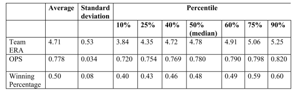
You have collected data from Major League Baseball (MLB)to find the determinants of winning.You have a general idea that both good pitching and strong hitting are needed to do well.However, you do not know how much each of these contributes separately.To investigate this problem, you collect data for all MLB during 1999 season.Your strategy is to first regress the winning percentage on pitching quality ("Team ERA"), second to regress the same variable on some measure of hitting ("OPS - On-base Plus Slugging percentage"), and third to regress the winning percentage on both. $\text {Summary of the Distribution of Winning Percentage, On Base plus}$ $\text {Slugging percentage, and Team Earned Run Average for MLB in 1999}$ $\text {The results are as follows:}$ = 0.94-0.100\times teamera ,=0.49, SER =0.06. (0.08)(0.017) = -0.68+1.513\times ops ,=0.45, SER =0.06. (0.17)(0.221) = -0.19-0.099\times teamera + (0.08)(0.008)(0.126) (a)Use the t-statistic to test for the statistical significance of the coefficient.

The Solow growth model suggests that countries with identical saving rates and population growth rates should converge to the same per capita income level. This result has been extended to include investment in human capital (education) as well as investment in physical capital. This hypothesis is referred to as the "conditional convergence hypothesis," since the convergence is dependent on countries obtaining the same values in the driving variables. To test the hypothesis, you collect data from the Penn World Tables on the average annual growth rate of GDP per worker $( \mathrm { g } 6090 )$ for the 1960-1990 sample period, and regress it on the (i) initial starting level of GDP per worker relative to the United States in 1960 (RelProd $_ { 60 }$ ), (ii) average population growth rate of the country $( n )$ , (iii) average investment share of GDP from 1960 to $1990 \left( s _ { \mathrm { K } } \right.$ - remember investment equals savings), and (iv) educational attainment in years for $1985 ( E d u c )$ . The results for close to 100 countries is as follows (numbers in parentheses are for heteroskedasticity-robust standard errors): =0.004-0.172\timesn+0.133\times+0.002\times Educ -0.044\times (0.007)(0.209)(0.015)(0.001)(0.008) =0.537,SER=0.011 (a)Is the coefficient on this variable significantly different from zero at the 5% level? At the 1% level?

If the estimates of the coefficients of interest change substantially across specifications,

The $F$ -statistic with $q = 2$ restrictions when testing for the restrictions $\beta _ { 1 } = 0$ and $\beta _ { 2 } = 0$ is given by the following formula: $F = \frac { 1 } { 2 } \left( \frac { t _ { 1 } ^ { 2 } + t _ { 2 } ^ { 2 } - 2 \hat { \rho } _ { t _ { 1 } , t _ { 2 } } t _ { 1 } t } { 1 - \hat { \rho } _ { t _ { 1 } , t _ { 2 } } ^ { 2 } } \right)$ Discuss how this formula can be understood intuitively.

When your multiple regression function includes a single omitted variable regressor, then

All of the following are true, with the exception of one condition: a. a high $R ^ { 2 }$ or $\bar { R } ^ { 2 }$ does not mean that the regressors are a true cause of the dependent variable. b. a high $R ^ { 2 }$ or $\bar { R } ^ { 2 }$ does not mean that there is no omitted variable bias. c. a high $R ^ { 2 }$ or $\bar { R } ^ { 2 }$ always means that an added variable is statistically significant. d. a high $R ^ { 2 }$ or $\bar { R } ^ { 2 }$ does not necessarily mean that you have the most appropriate set of regressors.

When testing the null hypothesis that two regression slopes are zero simultaneously, then you cannot reject the null hypothesis at the 5% level, if the ellipse contains the point a. $( - 1.96,1.96 )$ . b. $| ( 0,1.96 ) |$ . c. $( 0,0 )$ . d. $\left( 1.96 ^ { 2 } , 1.96 ^ { 2 } \right)$ .

The formula for the standard error of the regression coefficient, when moving from one explanatory variable to two explanatory variables,

If you wanted to test, using a 5 % significance level, whether or not a specific slope coefficient is equal to one, then you should

The overall regression F-statistic tests the null hypothesis that

To test joint linear hypotheses in the multiple regression model, you need to a. compare the sums of squared residuals from the restricted and unrestricted model. b. use the heteroskedasticity-robust $F$ -statistic. c. use several $t$ -statistics and perform tests using the standard normal distribution. d. compare the adjusted $R ^ { 2 }$ for the model which imposes the restrictions, and the unrestricted model.

Consider a situation where economic theory suggests that you impose certain restrictions on your estimated multiple regression function.These may involve the equality of parameters, such as the returns to education and on the job training in earnings functions, or the sum of coefficients, such as constant returns to scale in a production function.To test the validity of your restrictions, you have your statistical package calculate the corresponding F-statistic.Find the critical value from the F-distribution at the 5% and 1% level, and comment whether or not you will reject the null hypothesis in each of the following cases. (a)number of observations: 152; number of restrictions: 3; F-statistic: 3.21

Adding the Percent of English Speakers (PctEL)to the Student Teacher Ratio (STR)in your textbook reduced the coefficient for STR from 2.28 to 1.10 with a standard error of 0.43.Construct a 90% and 99% confidence interval to test the hypothesis that the coefficient of STR is 2.28.

Trying to remember the formula for the homoskedasticity-only F-statistic, you forgot whether you subtract the restricted SSR from the unrestricted SSR or the other way around.Your professor has provided you with a table containing critical values for the F distribution.How can this be of help?

All of the following are correct formulae for the homoskedasticity-only F-statistic, with the exception of a. $\quad F = \frac { \left( S S R _ { \text {restricted } } - S S R _ { \text {unrestricted } } \right) / q } { S S R _ { \text {unrestricted } } / \left( n - k _ { \text {unrestricted } } - 1 \right) }$ . b. $\quad F = \frac { \left( S S R _ { \text {unrestricted } } - S S R _ { \text {restricted } } \right) / q } { S S R _ { \text {restricted } } / \left( n - k _ { \text {restricted } } - 1 \right) }$ . c. $\quad F = \frac { \left( S S R _ { \text {restricted } } - S S R _ { \text {unrestricted } } \right) } { S S R _ { \text {unrestricted } } } \times \frac { n - k _ { \text {unrestricted } } - 1 } { q }$ . d. $\quad F = \left( \frac { S S R _ { \text {restricted } } } { S S R _ { \text {unrestricted } } } - 1 \right) \times \frac { \left( n - k _ { \text {unrestricted } } - 1 \right) } { q }$ . 1

The OLS estimators of the coefficients in multiple regression will have omitted variable bias a. only if an omitted determinant of $Y _ { i }$ is a continuous variable. b. if an omitted variable is correlated with at least one of the regressors, even though it is not a determinant of the dependent variable. c. only if the omitted variable is not normally distributed. d. if an omitted determinant of $Y _ { i }$ is correlated with at least one of the regressors.

In the multiple regression model, the t-statistic for testing that the slope is significantly different from zero is calculated a. by dividing the estimate by its standard error. b. from the square root of the $F$ -statistic. c. by multiplying the $p$ -value by $1.96$ . d. using the adjusted $R ^ { 2 }$ and the confidence interval.

Consider the following Cobb-Douglas production function $Y _ { i } = A K _ { i } ^ { \beta _ { 1 } } L _ { i } ^ { \beta _ { 2 } } e ^ { u _ { i } }$ (where Y is output, A is the level of technology, K is the capital stock, and L is the labor force), which has been linearized here (by using logarithms) to look as follows: $y _ { i } = \beta _ { 0 } ^ { * } + \beta _ { 1 } k _ { i } + \beta _ { 2 } l _ { i } + u _ { i }$ Assuming that the errors are heteroskedastic, you want to test for constant returns to scale. Using a t -statistic and "Approach #2," how would you proceed.