Exam 15: Estimation of Dynamic Causal Effects

The distributed lag model assumptions include all of the following with the exception of a. there is no perfect multicollinearity. b. $X _ { t }$ is strictly exogenous. c. $E \left( u _ { t } \mid X _ { t } , X _ { t - 1 } , X _ { t - 2 } , \ldots \right) = 0$ . d. The random variables $X _ { t }$ and $Y _ { t }$ have a stationary distribution.

In the distributed lag model, the coefficient on the contemporaneous value of the regressor is called the

It has been argued that Canada's aggregate output growth and unemployment rates are very sensitive to United States economic fluctuations, while the opposite is not true. (a)A researcher uses a distributed lag model to estimate dynamic causal effects of U.S. economic activity on Canada.The results (HAC standard errors in parenthesis)for the sample period 1961:I-1995:IV are: 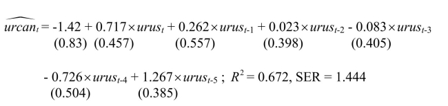where urcan is the Canadian unemployment rate, and urus is the United States unemployment rate. Calculate the long-run cumulative dynamic multiplier.

Autocorrelation of the error terms

A model that attracted quite a bit of interest in macroeconomics in the 1970s was the St. Louis model.The underlying idea was to calculate fiscal and monetary impact and long run cumulative dynamic multipliers, by relating output (growth)to government expenditure (growth)and money supply (growth).The assumption was that both government expenditures and the money supply were exogenous.Estimation of a St. Louis type model using quarterly data from 1960:I-1995:IV results in the following output (HAC standard errors in parenthesis): 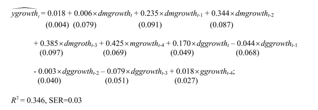where ygrowth is quarterly growth of real GDP, mgrowth is quarterly growth of real money supply (M2), and ggrowth is quarterly growth of real government expenditures. "d" in front of ggrowth and mgrowth indicates a change in the variable. (a)Assuming that money and government expenditures are exogenous, what do the coefficients represent? Calculate the h-period cumulative dynamic multipliers from these. How can you test for the statistical significance of the cumulative dynamic multipliers and the long-run cumulative dynamic multiplier?

The impact effect is the a. zero period dynamic multiplier. b. $h$ period dynamic multiplier, $h > 0$ . c. cumulative dynamic multiplier. d. long-run cumulative dynamic multiplier.

Your textbook mentions heteroskedasticity- and autocorrelation- consistent standard errors.Explain why you should use this option in your regression package when estimating the distributed lag regression model.What are the properties of the OLS estimator in the presence of heteroskedasticity and autocorrelation in the error terms? Explain why it is likely to find autocorrelation in time series data.If the errors are autocorrelated, then why not simply adjust for autocorrelation by using some non-linear estimation method such as Cochrane-Orcutt?

GLS

In time series, the definition of causal effects

To convey information about the dynamic multipliers more effectively, you should

In the distributed lag model, the dynamic causal effect

A distributed lag regression a. is also called $\operatorname { AR } ( p )$ . b. can also be used with cross-sectional data. c. gives estimates of dynamic causal effects. d. is sometimes referred to as ADL.

Heteroskedasticity- and autocorrelation-consistent standard errors

A seasonal binary (or indicator or dummy)variable, in the case of monthly data,

Your textbook presents as an example of a distributed lag regression the effect of the weather on the price of orange juice.The authors mention U.S.income and Australian exports, oil prices and inflation, monetary policy and inflation, and the Phillips curve as other candidates for distributed lag regression.Briefly discuss whether or not the exogeneity assumption is likely to hold in each of these cases.Explain why it is so hard to come up with good examples of distributed lag regressions in economics.

The distributed lag model is given by a. $Y _ { t } = \beta _ { 0 } + \beta _ { 1 } X _ { t } + \beta _ { 2 } Y _ { t - 1 } + u _ { t }$ . b. $Y _ { t } = \beta _ { 0 } + \beta _ { 1 } Y _ { t - 1 } + \beta _ { 2 } Y _ { t - 2 } + \ldots + \beta _ { r } Y _ { t - r } + u _ { t }$ . c. $Y _ { t } = \beta _ { 0 } + \beta _ { 1 } u _ { t } + \beta _ { 2 } u _ { t + 1 } + \beta _ { 3 } u _ { t + 2 } + \ldots + \beta _ { r + 1 } u _ { t + r } + e _ { t }$ . d. $Y _ { t } = \beta _ { 0 } + \beta _ { 1 } X _ { t } + \beta _ { 2 } X _ { t - 1 } + \beta _ { 3 } X _ { t - 2 } + \ldots + \beta _ { r + 1 } X _ { t - r } + u _ { t }$ .

Quasi differences in Yt are defined as a. $\quad Y _ { t } - Y _ { t - 1 }$ . b. $Y _ { t } - \phi _ { 1 } Y _ { t - 1 }$ . c. $\Delta Y _ { t } - \phi _ { 1 } Y _ { t - 1 }$ . d. $\quad \phi _ { 1 } \left( Y _ { t } - Y _ { t - 1 } \right)$ .

In your intermediate macroeconomics course, government expenditures and the money supply were treated as exogenous, in the sense that the variables could be changed to conduct economic policy to influence target variables, but that these variables would not react to changes in the economy as a result of some fixed rule.The St.Louis Model, proposed by two researchers at the Federal Reserve in St.Louis, used this idea to test whether monetary policy or fiscal policy was more effective in influencing output behavior.Although there were various versions of this model, the basic specification was of the following type: $\Delta \ln \left( Y _ { t } \right) = \beta _ { 0 } + \beta _ { 1 } \Delta \ln m _ { t } + \ldots + \beta _ { p } \Delta \ln m _ { t - p - 1 } + \beta _ { p + 1 } \Delta \ln G _ { t } + \ldots + \beta _ { p + q } \Delta \ln G _ { t - q - 1 } + u _ { t }$ Assuming that money supply and government expenditures are exogenous, how would you estimate dynamic causal effects? Why do you think this type of model is no longer used by most to calculate fiscal and monetary multipliers?

One of the central predictions of neo-classical macroeconomic growth theory is that an increase in the growth rate of the population causes at first a decline the growth rate of real output per capita, but that subsequently the growth rate returns to its natural level, itself determined by the rate of technological innovation.The intuition is that, if the growth rate of the workforce increases, then more has to be saved to provide the new workers with physical capital.However, accumulating capital takes time, so that output per capita falls in the short run. Under the assumption that population growth is exogenous, a number of regressions of the growth rate of output per capita on current and lagged population growth were performed, as reported below.(A constant was included in the regressions but is not reported.HAC standard errors are in brackets.BIC is listed at the bottom of the table). Regression of Growth Rate of Real Per-Capita GDP on Lags of Population Growth, United States, 1825-2000. Lag number Dynamic multipliers Dynamic multipliers Dynamic multipliers (1) Dynamic multipliers Dynamic multipliers 0 -0.9 -1.1 -1.3 -0.2 -2.0 (1.3) (1.3) (1.7) (1.7) (1.5) 1 3.5 3.2 1.8 0.8 - 2 (1.6) (1.6) (1.6) (1.5) - 3 -1.3 -3.0 -2.2 - - 4 (1.7) 1.6) (1.4) - - BIC -234.4 -236.1 -238.5 -240.0 -241.8 (a)Which of these models is favored by the information criterion?

The concept of exogeneity is important because