Exam 14: Introduction to Time Series Regression and Forecasting
Exam 1: Economic Questions and Data11 Questions
Exam 2: Review of Probability61 Questions
Exam 3: Review of Statistics56 Questions
Exam 4: Linear Regression With One Regressor54 Questions
Exam 5: Regression With a Single Regressor: Hypothesis Tests and Confidence Intervals53 Questions
Exam 6: Linear Regression With Multiple Regressors54 Questions
Exam 7: Hypothesis Tests and Confidence Intervals in Multiple Regression50 Questions
Exam 8: Nonlinear Regression Functions53 Questions
Exam 9: Assessing Studies Based on Multiple Regression55 Questions
Exam 10: Regression With Panel Data40 Questions
Exam 11: Regression With a Binary Dependent Variable40 Questions
Exam 12: Instrumental Variables Regression40 Questions
Exam 13: Experiments and Quasi-Experiments40 Questions
Exam 14: Introduction to Time Series Regression and Forecasting36 Questions
Exam 15: Estimation of Dynamic Causal Effects40 Questions
Exam 16: Additional Topics in Time Series Regression40 Questions
Exam 17: The Theory of Linear Regression With One Regressor39 Questions
Exam 18: The Theory of Multiple Regression38 Questions
Select questions type
An autoregression is a regression
Free
(Multiple Choice)
4.8/5  (30)
(30)
Correct Answer: Verified
C
To choose the number of lags in either an autoregression or in a time series regression model with multiple predictors, you can use any of the following test statistics with the
Exception of the
Free
(Multiple Choice)
4.8/5 (42)
Correct Answer:Verified
D
(Requires Appendix Material) Define the difference operator , where is the lag operator, such that . In general, , where and are typically omitted when they take the value of 1. Show the expressions in only when applying the difference operator to the following expressions, and give the resulting expression an economic interpretation, assuming that you are working with quarterly data: (a)
Free
(Essay)
4.9/5 (37)
Correct Answer:Verified
This represents the change in the annual change.If Y is in logarithms, then this
is the change in the annual growth rate.
(Requires Appendix material): Show that the AR(1) process
be converted to a process.
(Essay)
4.7/5 (40)
The time interval between observations can be all of the following with the exception of data collected
(Multiple Choice)
4.8/5 (34)
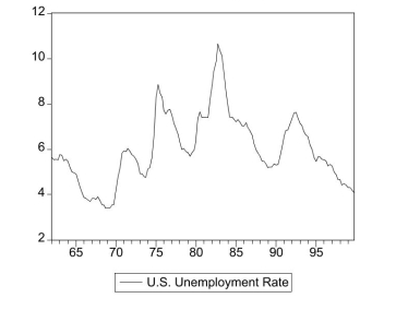
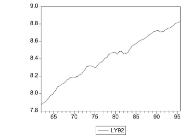
The following two graphs give you a plot of the United States aggregate unemployment
rate for the sample period 1962:I to 1999:IV, and the (log)level of real United States
GDP for the sample period 1962:I to 1995:IV.You want test for stationarity in both
cases.Indicate whether or not you should include a time trend in your Augmented
Dickey-Fuller test and why. United States Unemployment Rate
 United States Real GDP (in logarithms)
(Essay)
4.9/5 (33)
Consider the following model t
where the superscript "e" indicates expected values.This may represent an example
where consumption depended on expected, or "permanent," income.Furthermore, let
expected income be formed as follows: 1
This particular type of expectation formation is called the "adaptive expectations
hypothesis."
(a) In the above expectation formation hypothesis, expectations are formed at the beginning of the period, say the of January if you had annual data. Give an intuitive explanation for this process.
(Essay)
5.0/5 (31)
(Requires Appendix material) The long-run, stationary state solution of an model, which can be written as , where , and , , can be found by setting in the two lag polynomials. Explain. Derive the long-run solution for the estimated of the change in the inflation rate on unemployment: =1.32-.36\Delta Inf -0.34\Delta+.07\Delta Inf -.03\Delta Inf -2.68+3.43-1.04+.07 Assume that the inflation rate is constant in the long-run and calculate the resulting
unemployment rate.What does the solution represent? Is it reasonable to assume that this
long-run solution is constant over the estimation period 1962-1999? If not, how could
you detect the instability?
(Essay)
4.9/5 (45)
Pseudo out of sample forecasting can be used for the following reasons with the exception of
(Multiple Choice)
4.7/5 (42)
You have decided to use the Dickey Fuller (DF)test on the United States aggregate
unemployment rate (sample period 1962:I - 1995:IV).As a result, you estimate the
following AR(1)model = 0.114-0.024,=0.0118, SER =0.3417 (0.121)(0.019)
You recall that your textbook mentioned that this form of the AR(1)is convenient
because it allows for you to test for the presence of a unit root by using the t- statistic of
the slope.Being adventurous, you decide to estimate the original form of the AR(1)
instead, which results in the following output = 0.114-0.024,=0.0118, SER =0.3417 (0.121)(0.019)
You are surprised to find the constant, the standard errors of the two coefficients, and the SER unchanged, while the regression increased substantially. Explain this increase in the regression . Why should you have been able to predict the change in the slope coefficient and the constancy of the standard errors of the two coefficients and the SER?
(Essay)
4.7/5 (36)
You set out to forecast the unemployment rate in the United States (UrateUS), using
quarterly data from 1960, first quarter, to 1999, fourth quarter.
(a)The following table presents the first four autocorrelations for the United States
aggregate unemployment rate and its change for the time period 1960 (first quarter)to
1999 (fourth quarter).Explain briefly what these two autocorrelations measure. First Four Autocorrelations of the U.S. Unemployment Rate and its Change,
1960:I - 1999 IV
Unemployment Rate Change of Unemployment Rate 1 0.97 0.62 2 0.92 0.32 3 0.83 0.12 4 0.75 -0.07
(Essay)
4.8/5 (36)
The textbook displayed the accompanying four economic time series with "markedly
different patterns." For each indicate what you think the sample autocorrelations of the
level (Y)and change ( ΔY )will be and explain your reasoning.
(a) 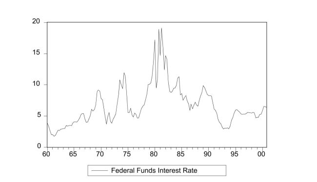
(Essay)
4.9/5 (42)
Problems caused by stochastic trends include all of the following with the exception of
(Multiple Choice)
4.9/5 (35)
You collect monthly data on the money supply (M2) for the United States from 1962:12002:4 to forecast future money supply behavior.
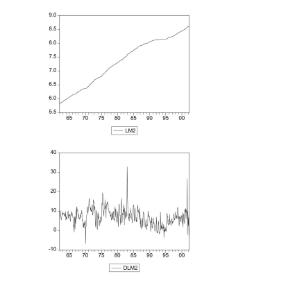 where and are the log level and growth rate of M2. (a)Using quarterly data, when analyzing inflation and unemployment in the United States,
the textbook converted log levels of variables into growth rates by differencing the log
levels, and then multiplying these by 400.Given that you have monthly data, how would
you proceed here?
where and are the log level and growth rate of M2. (a)Using quarterly data, when analyzing inflation and unemployment in the United States,
the textbook converted log levels of variables into growth rates by differencing the log
levels, and then multiplying these by 400.Given that you have monthly data, how would
you proceed here?
(Essay)
4.8/5 (36)
Filters
- Essay(0)
- Multiple Choice(0)
- Short Answer(0)
- True False(0)
- Matching(0)