Exam 4: Linear Regression With One Regressor

Multiplying the dependent variable by 100 and the explanatory variable by 100,000 leaves the a. OLS estimate of the slope the same. b. OLS estimate of the intercept the same. c. regression $R ^ { 2 }$ the same. d. variance of the OLS estimators the same.

$\mathrm { E } \left( u _ { i } \mid X _ { i } \right) = 0$ says that

When the estimated slope coefficient in the simple regression model, $\hat { \beta } _ { 1 } ,$ is zero, then

Assume that there is a change in the units of measurement on X . The new variables $X ^ { * } = b X \text {. }$ Prove that this change in the units of measurement on the explanatory variable has no effect on the intercept in the resulting regression.

The neoclassical growth model predicts that for identical savings rates and population growth rates, countries should converge to the per capita income level.This is referred to as the convergence hypothesis.One way to test for the presence of convergence is to compare the growth rates over time to the initial starting level. (a)If you regressed the average growth rate over a time period (1960-1990)on the initial level of per capita income, what would the sign of the slope have to be to indicate this type of convergence? Explain.Would this result confirm or reject the prediction of the neoclassical growth model?

Show first that the regression $R ^ { 2 }$ is the square of the sample correlation coefficient. Next, show that the slope of a simple regression of Y on X is only identical to the inverse of the regression slope of X on Y if the regression $R ^ { 2 }$ equals one.

Sir Francis Galton, a cousin of James Darwin, examined the relationship between the height of children and their parents towards the end of the 19th century.It is from this study that the name "regression" originated.You decide to update his findings by collecting data from 110 college students, and estimate the following relationship: $\widehat { \text { Studenth } } = 19.6 + 0.73 \times \text { Midparh, } R ^ { 2 } = 0.45 , S E R = 2.0$ where Studenth is the height of students in inches, and Midparh is the average of the parental heights.(Following Galton's methodology, both variables were adjusted so that the average female height was equal to the average male height.) (a)Interpret the estimated coefficients.

You have obtained a sub-sample of 1744 individuals from the Current Population Survey (CPS)and are interested in the relationship between weekly earnings and age.The regression, using heteroskedasticity-robust standard errors, yielded the following result: $\widehat { \text { Earn } } = 239.16 + 5.20 \times \text { Age } , R ^ { 2 } = 0.05 , \text { SER } = 287.21 .$ where Earn and Age are measured in dollars and years respectively. (a)Interpret the results.

The standard error of the regression (SER) is defined as follows

You have learned in one of your economics courses that one of the determinants of per capita income (the "Wealth of Nations")is the population growth rate.Furthermore you also found out that the Penn World Tables contain income and population data for 104 countries of the world.To test this theory, you regress the GDP per worker (relative to the United States)in 1990 (RelPersInc)on the difference between the average population growth rate of that country (n)to the U.S.average population growth rate (nus )for the years 1980 to 1990.This results in the following regression output: $\widehat { \text { RelPersInc } } = 0.518 - 18.831 \times \left( n - n _ { u s } \right) , R ^ { 2 } = 0.522 , S E R = 0.197$ (a)Interpret the results carefully.Is this relationship economically important?

The news-magazine The Economist regularly publishes data on the so called Big Mac index and exchange rates between countries.The data for 30 countries from the April 29, 2000 issue is listed below: 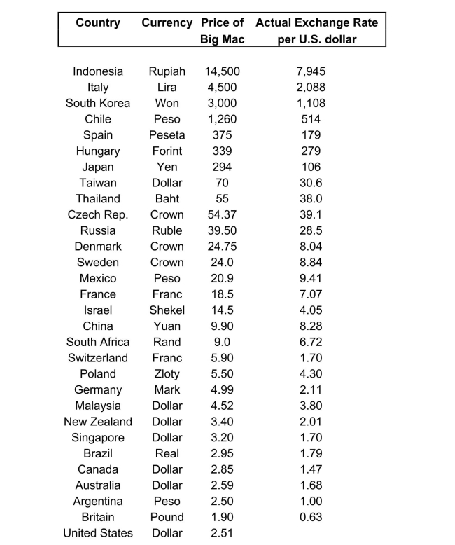The concept of purchasing power parity or PPP ("the idea that similar foreign and domestic goods ... should have the same price in terms of the same currency," Abel, A. and B. Bernanke, Macroeconomics, $4 ^ { \text {th } }$ edition, Boston: Addison Wesley, 476) suggests that the ratio of the Big Mac priced in the local currency to the U.S. dollar price should equal the exchange rate between the two countries. a)Enter the data into your regression analysis program (EViews, Stata, Excel, SAS, etc.). Calculate the predicted exchange rate per U.S.dollar by dividing the price of a Big Mac in local currency by the U.S.price of a Big Mac ($2.51).

(Requires Appendix material)Show that the two alternative formulae for the slope given in your textbook are identical. $\frac { \frac { 1 } { n } \sum _ { i = 1 } ^ { n } X _ { i } Y _ { i } - \bar { X } \bar { Y } } { \frac { 1 } { n } \sum _ { i = 1 } ^ { n } X _ { i } ^ { 2 } - \bar { X } ^ { 2 } } = \frac { \sum _ { i = 1 } ^ { n } \left( X _ { i } - \bar { X } \right) \left( Y _ { i } - \bar { Y } \right) } { \sum _ { i = 1 } ^ { n } \left( X _ { i } - \bar { X } \right) ^ { 2 } }$

The variance of $Y _ { i }$ is given by

(Requires Calculus)Consider the following model: $Y _ { i } = \beta _ { 1 } X _ { i } + u _ { i }$ $\text { Derive the OLS estimator for } \beta _ { 1 } \text {. }$

The normal approximation to the sampling distribution of $\widehat { \beta } _ { 1 }$ is powerful because

In 2001, the Arizona Diamondbacks defeated the New York Yankees in the Baseball World Series in 7 games.Some players, such as Bautista and Finley for the Diamondbacks, had a substantially higher batting average during the World Series than during the regular season.Others, such as Brosius and Jeter for the Yankees, did substantially poorer.You set out to investigate whether or not the regular season batting average is a good indicator for the World Series batting average.The results for 11 players who had the most at bats for the two teams are: =-0.347+2.290 AZSeasavg ,=0.11, SER =0.145, =0.134+0.136 NYSeasavg ,=0.001, SER =0.092, where Wsavg and Seasavg indicate the batting average during the World Series and the regular season respectively. (a)Focusing on the coefficients first, what is your interpretation?

The OLS residuals

(Requires Appendix material) The sample regression line estimated by OLS

(Requires Appendix material) Which of the following statements is correct?

A peer of yours, who is a major in another social science, says he is not interested in the regression slope and/or intercept.Instead he only cares about correlations.For example, in the testscore/student-teacher ratio regression, he claims to get all the information he needs from the negative correlation coefficient corr(X,Y)=-0.226.What response might you have for your peer?