Exam 16: Time-Series Forecasting

SCENARIO 16-13 Given below is the monthly time series data for U.S. retail sales of building materials over a specific year. Month Retail Sales 1 6,594 2 6,610 3 8,174 4 9,513 5 10,595 6 10,415 7 9,949 8 9,810 9 9,637 10 9,732 11 9,214 12 9,201 The results of the linear trend, quadratic trend, exponential trend, first-order autoregressive, second-order autoregressive and third-order autoregressive model are presented below in which the coded month for the 1st month is 0: $\text { Linear trend model: }$ Coefficients Standard Error t Stat P-value Intercept 7950.7564 617.6342 12.8729 0.0000 Coded Month 212.6503 95.1145 2.2357 0.0494 $\text { Quadratic trend model: }$ $\text { Exponential trend model: }$ Coefficients Standard Error t Stat P-value Intercept 3.8912 0.0315 123.3674 0.0000 Coded Month 0.0116 0.0049 2.3957 0.0376 $\text { First-order autoregressive: }$ Coefficients Standard Error t Stat P-value Intercept 3132.0951 1287.2899 2.4331 0.0378 YLag1 0.6823 0.1398 4.8812 0.0009 -Referring to Scenario 16-13, what is the p-value of the t test statistic for testing the appropriateness of the third-order autoregressive model?

SCENARIO 16-15-A You are the CEO of a diary company. The total milk production (in gallons) from your company over the past 30 years are presented below and also contained in the Excel file SCENARIO 16- 15-A.XLSX. Year 1986 1987 1988 1989 1990 1991 1992 1993 1994 1995 1996 1997 1998 1999 2000 2001 2002 2003 2004 2005 2006 2007 2008 2009 2010 2011 2012 2013 2014 2015 Milk 150201 172719 171357 157121 155727 152974 153443 158548 162614 164210 Prod 159127 153866 165992 177843 167477 163821 161700 170348 174105 185103 184670 173385 159695 173641 165706 171164 168706 150684 179314 163802 You want to predict your company's future total milk production using the linear trend, quadratic trend, exponential trend, first-order autoregressive, second-order autoregressive and third-order autoregressive model. -Referring to Scenario 16-15-A, what is the exponentially smoothed value for 1986 using a smoothing coefficient of W = 0.5?

SCENARIO 16-11 The manager of a health club has recorded mean attendance in newly introduced step classes over the last 15 months: 32.1, 39.5, 40.3, 46.0, 65.2, 73.1, 83.7, 106.8, 118.0, 133.1, 163.3, 182.8, 205.6, 249.1, and 263.5. She then used Microsoft Excel to obtain the following partial output for both a first- and second-order autoregressive model. 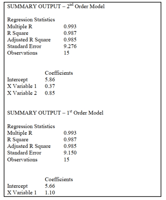-Referring to Scenario 16-11, using the second-order model, the forecast of mean attendance for month 17 is __________.

SCENARIO 16-13 Given below is the monthly time series data for U.S. retail sales of building materials over a specific year. Month Retail Sales 1 6,594 2 6,610 3 8,174 4 9,513 5 10,595 6 10,415 7 9,949 8 9,810 9 9,637 10 9,732 11 9,214 12 9,201 The results of the linear trend, quadratic trend, exponential trend, first-order autoregressive, second-order autoregressive and third-order autoregressive model are presented below in which the coded month for the 1st month is 0: $\text { Linear trend model: }$ Coefficients Standard Error t Stat P-value Intercept 7950.7564 617.6342 12.8729 0.0000 Coded Month 212.6503 95.1145 2.2357 0.0494 $\text { Quadratic trend model: }$ $\text { Exponential trend model: }$ Coefficients Standard Error t Stat P-value Intercept 3.8912 0.0315 123.3674 0.0000 Coded Month 0.0116 0.0049 2.3957 0.0376 $\text { First-order autoregressive: }$ Coefficients Standard Error t Stat P-value Intercept 3132.0951 1287.2899 2.4331 0.0378 YLag1 0.6823 0.1398 4.8812 0.0009 -Referring to Scenario 16-13, the best model based on the residual plots is the exponential-trend regression model.

SCENARIO 16-15-B You are the CEO of a diary company. The total milk production (in gallons) from your company over the past 30 years are presented below and also contained in the Excel file SCENARIO 16- 15-B.XLSX. Year 1986 1987 1988 1989 1990 1991 1992 1993 1994 1995 1996 1997 1998 1999 2000 2001 2002 2003 2004 2005 2006 2007 2008 2009 2010 2011 2012 2013 2014 2015 Milk 150201 193718 212520 214553 237507 248069 241824 234627 252049 252029 Prod 263449 260689 247900 260059 268197 249477 246216 265236 256364 241705 245932 243529 241551 247697 248454 241974 235823 243517 238490 248606 You want to predict your company's future total milk production using the linear trend, quadratic trend, exponential trend, first-order autoregressive, second-order autoregressive and third-order autoregressive model. -Referring to Scenario 16-15-B, you can conclude that the quadratic term in the quadratic-trend model is statistically significant at the 5% level of significance.

SCENARIO 16-2 The monthly advertising expenditures of a department store chain (in $1,000,000s) were collected over the last decade. The last 14 months of this time series follows: $\begin{array} { c l } \text { Month } & \text { Expenditures (\$) } \\\hline 1 & 1.4 \\2 & 1.8 \\3 & 1.6 \\4 & 1.5 \\5 & 1.8 \\6 & 1.7 \\7 & 1.9 \\8 & 2.2 \\9 & 1.9 \\10 & 1.9 \\11 & 2.1 \\12 & 2.4 \\13 & 2.8 \\14 & 3.1\end{array}$ -Referring to Scenario 16-2, advertising expenditures appear to be increasing in a linear rather than curvilinear manner over time.

SCENARIO 16-14 A contractor developed a multiplicative time-series model to forecast the number of contracts in future quarters, using quarterly data on number of contracts during the 3-year period from 2011 to -Referring to Scenario 16-14, using the regression equation, which of the following values is the best forecast for the number of contracts in the third quarter of 2014?

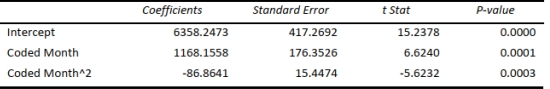
SCENARIO 16-13 Given below is the monthly time series data for U.S. retail sales of building materials over a specific year. Month Retail Sales 1 6,594 2 6,610 3 8,174 4 9,513 5 10,595 6 10,415 7 9,949 8 9,810 9 9,637 10 9,732 11 9,214 12 9,201 The results of the linear trend, quadratic trend, exponential trend, first-order autoregressive, second-order autoregressive and third-order autoregressive model are presented below in which the coded month for the 1st month is 0: $\text { Linear trend model: }$ Coefficients Standard Error t Stat P-value Intercept 7950.7564 617.6342 12.8729 0.0000 Coded Month 212.6503 95.1145 2.2357 0.0494 $\text { Quadratic trend model: }$ $\text { Exponential trend model: }$ Coefficients Standard Error t Stat P-value Intercept 3.8912 0.0315 123.3674 0.0000 Coded Month 0.0116 0.0049 2.3957 0.0376 $\text { First-order autoregressive: }$ Coefficients Standard Error t Stat P-value Intercept 3132.0951 1287.2899 2.4331 0.0378 YLag1 0.6823 0.1398 4.8812 0.0009 -Referring to Scenario 16-13, what is the exponentially smoothed value for the first month using a smoothing coefficient of W = 0.25?

SCENARIO 16-3 The following table contains the number of complaints received in a department store for the first 6 months of last year. Month Complaints January 36 February 45 March 81 April 90 May 108 June 144 -If you want to recover the trend using exponential smoothing, you will choose a weight (W) that falls in the range

SCENARIO 16-8 The manager of a marketing consulting firm has been examining his company's yearly profits. He believes that these profits have been showing a quadratic trend since 1994. He uses Microsoft Excel to obtain the partial output below. The dependent variable is profit (in thousands of dollars), while the independent variables are coded years and squared of coded years, where 1994 is coded as 0, 1995 is coded as 1, etc. -Referring to Scenario 16-8, the forecast for profits in 2019 is __________.

SCENARIO 16-3 The following table contains the number of complaints received in a department store for the first 6 months of last year. Month Complaints January 36 February 45 March 81 April 90 May 108 June 144 -Referring to Scenario 16-3, if this series is smoothed using exponential smoothing with a smoothing constant of 1/3, what would be the first value?

When using the exponentially weighted moving average for purposes of forecasting rather than smoothing,

SCENARIO 16-15-A You are the CEO of a diary company. The total milk production (in gallons) from your company over the past 30 years are presented below and also contained in the Excel file SCENARIO 16- 15-A.XLSX. Year 1986 1987 1988 1989 1990 1991 1992 1993 1994 1995 1996 1997 1998 1999 2000 2001 2002 2003 2004 2005 2006 2007 2008 2009 2010 2011 2012 2013 2014 2015 Milk 150201 172719 171357 157121 155727 152974 153443 158548 162614 164210 Prod 159127 153866 165992 177843 167477 163821 161700 170348 174105 185103 184670 173385 159695 173641 165706 171164 168706 150684 179314 163802 You want to predict your company's future total milk production using the linear trend, quadratic trend, exponential trend, first-order autoregressive, second-order autoregressive and third-order autoregressive model. -Referring to Scenario 16-15-A, what is the value of the t test statistic for testing the significance of the quadratic term in the quadratic-trend model?

SCENARIO 16-12 A local store developed a multiplicative time-series model to forecast its revenues in future quarters, using quarterly data on its revenues during the 5-year period from 2009 to 2013. The following is the resulting regression equation: $\log _ { 10 } \hat { Y } = 6.102 + 0.012 X - 0.129 Q _ { 1 } - 0.054 Q _ { 2 } + 0.098 Q _ { 3 }$ where $\hat { Y }$ is the estimated number of contracts in a quarter $X$ is the coded quarterly value with $X = 0$ in the first quarter of 2008 . $Q _ { 1 }$ is a dummy variable equal to 1 in the first quarter of a year and 0 otherwise. $Q _ { 2 }$ is a dummy variable equal to 1 in the second quarter of a year and 0 otherwise. $Q _ { 3 }$ is a dummy variable equal to 1 in the third quarter of a year and 0 otherwise. -Referring to Scenario 16-12, the best interpretation of the constant 6.102 in the regression equation is: a) the fitted value for the first quarter of 2009 , prior to seasonal adjustment, is $\log _ { 10 } ( 6.102 )$ . b) the fitted value for the first quarter of 2009 , after to seasonal adjustment, is $\log _ { 10 } ( 6.102 )$ . c) the fitted value for the first quarter of 2009 , prior to seasonal adjustment, is $10 ^ { 6.102 }$ . d) the fitted value for the first quarter of 2009 , after to seasonal adjustment, is $10 ^ { 6.102 }$ .

The method of least squares may be used to estimate both linear and curvilinear trends.