Exam 7: Inference When Variables Are Related
For a class project, students tested four different brands of laundry detergent (1, 2, 3, 4) in
three different water temperatures (hot, warm, cold) to see whether their were any
differences in how well the detergents could clean clothes. The students took 36 identical
pieces of cloth and made them dirty by staining them with coffee, dirt, and grass. The 36
pieces were randomly assigned to the 12 combinations of detergent and temperature so
that each combination had 3 replicates. After washing, the students rated how clean the
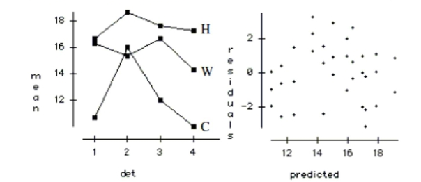
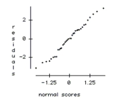
clothes were from 0 (no change) to 20 (completely spotless). The two factor ANOVA table
is shown below along with an interaction plot and residual plots. Source df Sums of Squares Mean Square F-ratio P-value Detergent 3 38.972 12.9907 3.966 0.0171 Temp 2 181.056 90.5278 27.634 <0.0001 Error 30 98.278 3.2759 Total 35 318.306
 a. Write the hypotheses tested by the Detergent F-ratio. Test the hypotheses and explain
your conclusion in the context of the problem.
b. Write the hypotheses tested by the Temp F-ratio. Test the hypotheses and explain your
conclusion in the context of the problem.
c. Check the conditions required for the ANOVA analysis.
a. Write the hypotheses tested by the Detergent F-ratio. Test the hypotheses and explain
your conclusion in the context of the problem.
b. Write the hypotheses tested by the Temp F-ratio. Test the hypotheses and explain your
conclusion in the context of the problem.
c. Check the conditions required for the ANOVA analysis.
a. . Each detergent has an equal effect on the how clean the clothes are.
: At least one detergent has a different effect than the others.
There is strong evidence that the detergents do not clean equally well.
b. Warm Cold. Each temperature has an equal effect on the how clean the clothes are.
: At least one temperature has a different effect than the others.
There is strong evidence that the temperatures do not clean equally well.
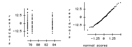
c. Randomization: OK. The treatments were applied to the clothes in a random order.
* Additive enough: Violated. The lines in the interaction plot are not parallel. It seems that Detergent 2 cleans much better than expected in cold water. Add an interaction term.
* Similar variance: Caution. The residual vs. predicted plot shows slightly uneven spread. However, the differences observed are so strong that should not affect our conclusions.
* Nearly normal: OK. The normal probability plot is straight.
Here are data about the average January low temperature in cities in the United States, and factors that might allow us to
predict temperature. The data, available for 55 cities, include:  We will attempt to make a regression model to help account for mean January temperature and to understand the effects of
the various predictors.
At each step of the analysis you may assume that things learned earlier in the process are known.
Units Note: The "degrees" of temperature, given here on the Fahrenheit scale, have only coincidental language relationship to
the "degrees" of longitude and latitude. The geographic "degrees" are based on modeling the Earth as a sphere and dividing it
up into 360 degrees for a full circle. Thus 180 degrees of longitude is halfway around the world from Greenwich, England
(0°) and Latitude increases from 0 degrees at the Equator to 90 degrees of (North) latitude at the North Pole.
We will attempt to make a regression model to help account for mean January temperature and to understand the effects of
the various predictors.
At each step of the analysis you may assume that things learned earlier in the process are known.
Units Note: The "degrees" of temperature, given here on the Fahrenheit scale, have only coincidental language relationship to
the "degrees" of longitude and latitude. The geographic "degrees" are based on modeling the Earth as a sphere and dividing it
up into 360 degrees for a full circle. Thus 180 degrees of longitude is halfway around the world from Greenwich, England
(0°) and Latitude increases from 0 degrees at the Equator to 90 degrees of (North) latitude at the North Pole. 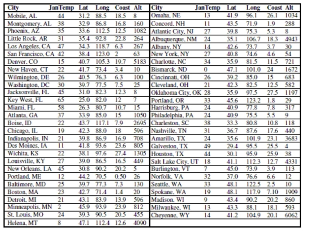 -It is possible that the distance that a city is from the ocean could affect its average January
low temperature. Coast gives an approximate distance of each city from the East Coast or
West Coast (whichever is nearer). Including it in the regression yields the following
regression table: Dependent variable is:JanTemp
R squared squared (adjusted) with degrees of freedom
Source Sum of Squares df Mean Square F-ratio Regression 8611.86 3 2870.62 121 Residual 1213.67 51 23.7974
Variable Coefficient SE ( Coeff ) t-ratio P-value Intercept 111.878 6.167 18.1 \leq0.0001 Lat -2.47722 0.1307 -19.0 \leq0.0001 Long 0.221997 0.0462 4.81 \leq0.0001 Coast -0.674929 0.0901 -7.49 \leq0.0001
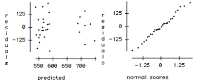
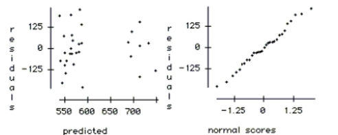
And here is a scatterplot of the residuals:
-It is possible that the distance that a city is from the ocean could affect its average January
low temperature. Coast gives an approximate distance of each city from the East Coast or
West Coast (whichever is nearer). Including it in the regression yields the following
regression table: Dependent variable is:JanTemp
R squared squared (adjusted) with degrees of freedom
Source Sum of Squares df Mean Square F-ratio Regression 8611.86 3 2870.62 121 Residual 1213.67 51 23.7974
Variable Coefficient SE ( Coeff ) t-ratio P-value Intercept 111.878 6.167 18.1 \leq0.0001 Lat -2.47722 0.1307 -19.0 \leq0.0001 Long 0.221997 0.0462 4.81 \leq0.0001 Coast -0.674929 0.0901 -7.49 \leq0.0001
And here is a scatterplot of the residuals: 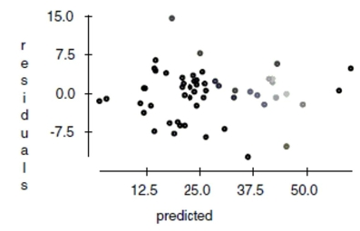
This regression model seems to be an improvement. The model accounts for 87.6%
of the variability in average January low temperatures and all the standard
hypothesis tests on the coefficients are highly significant. The residuals plot shows
no particular pattern of concern.
Here are data about the average January low temperature in cities in the United States, and factors that might allow us to
predict temperature. The data, available for 55 cities, include:  We will attempt to make a regression model to help account for mean January temperature and to understand the effects of
the various predictors.
At each step of the analysis you may assume that things learned earlier in the process are known.
Units Note: The "degrees" of temperature, given here on the Fahrenheit scale, have only coincidental language relationship to
the "degrees" of longitude and latitude. The geographic "degrees" are based on modeling the Earth as a sphere and dividing it
up into 360 degrees for a full circle. Thus 180 degrees of longitude is halfway around the world from Greenwich, England
(0°) and Latitude increases from 0 degrees at the Equator to 90 degrees of (North) latitude at the North Pole.
We will attempt to make a regression model to help account for mean January temperature and to understand the effects of
the various predictors.
At each step of the analysis you may assume that things learned earlier in the process are known.
Units Note: The "degrees" of temperature, given here on the Fahrenheit scale, have only coincidental language relationship to
the "degrees" of longitude and latitude. The geographic "degrees" are based on modeling the Earth as a sphere and dividing it
up into 360 degrees for a full circle. Thus 180 degrees of longitude is halfway around the world from Greenwich, England
(0°) and Latitude increases from 0 degrees at the Equator to 90 degrees of (North) latitude at the North Pole.  -Here is the regression with both Latitude and Longitude as predictors: Dependent variable is: JanTemp R squared R squared (adjusted)
with degrees of freedom
Source Sum of Squares df Mean Square F-ratio Regression 7277.18 2 3638.59 74.2 Residual 2548.35 52 49.0067 Variable Coefficient SE ( Coeff ) t-ratio P-value Intercept 98.5620 8.473 11.6 \leq0.0001 Lat -2.16286 0.1776 -12.2 \leq0.0001 Long 0.134471 0.0641 2.10 0.0407
The coefficient of Long in this regression differs from the coefficient of Long in the simple regression of JanTemp on Long. What is the meaning of the coefficient of Long in this regression? Are you confident (at ) that the coefficient is not zero? Why or why not?
-Here is the regression with both Latitude and Longitude as predictors: Dependent variable is: JanTemp R squared R squared (adjusted)
with degrees of freedom
Source Sum of Squares df Mean Square F-ratio Regression 7277.18 2 3638.59 74.2 Residual 2548.35 52 49.0067 Variable Coefficient SE ( Coeff ) t-ratio P-value Intercept 98.5620 8.473 11.6 \leq0.0001 Lat -2.16286 0.1776 -12.2 \leq0.0001 Long 0.134471 0.0641 2.10 0.0407
The coefficient of Long in this regression differs from the coefficient of Long in the simple regression of JanTemp on Long. What is the meaning of the coefficient of Long in this regression? Are you confident (at ) that the coefficient is not zero? Why or why not?
The coefficient of Long now measures the effect of longitude after allowing for the
effects of latitude on January temperature. With a P-value of 0.04 we can reject the
null hypothesis that this coefficient is zero at
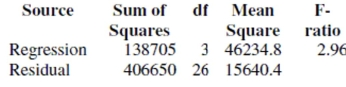
When a sum of squares is divided by its degrees of freedom, the result is called a(n)...
Here are data about the average January low temperature in cities in the United States, and factors that might allow us to
predict temperature. The data, available for 55 cities, include:  We will attempt to make a regression model to help account for mean January temperature and to understand the effects of
the various predictors.
At each step of the analysis you may assume that things learned earlier in the process are known.
Units Note: The "degrees" of temperature, given here on the Fahrenheit scale, have only coincidental language relationship to
the "degrees" of longitude and latitude. The geographic "degrees" are based on modeling the Earth as a sphere and dividing it
up into 360 degrees for a full circle. Thus 180 degrees of longitude is halfway around the world from Greenwich, England
(0°) and Latitude increases from 0 degrees at the Equator to 90 degrees of (North) latitude at the North Pole.
We will attempt to make a regression model to help account for mean January temperature and to understand the effects of
the various predictors.
At each step of the analysis you may assume that things learned earlier in the process are known.
Units Note: The "degrees" of temperature, given here on the Fahrenheit scale, have only coincidental language relationship to
the "degrees" of longitude and latitude. The geographic "degrees" are based on modeling the Earth as a sphere and dividing it
up into 360 degrees for a full circle. Thus 180 degrees of longitude is halfway around the world from Greenwich, England
(0°) and Latitude increases from 0 degrees at the Equator to 90 degrees of (North) latitude at the North Pole. 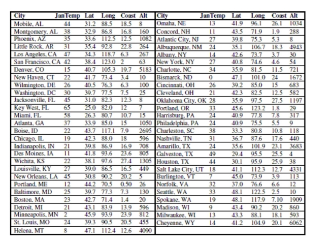 -Here is the corresponding regression table: Dependent variable is: JanTemp
squared squared (adjusted)
with degrees of freedom
Source Sum of Squares df Mean Square F-ratio Regression 7061.32 1 7061.32 135 Residual 2764.21 53 52.1549
Variable Coefficient SE(Coeff) t-ratio P-value Intercept 108.805 7.146 15.2 \leq0.0001 Lat -2.11114 0.1814 -11.6 \leq0.0001
Write a brief report based on this regression. Explain in words and numbers what this
equation says about the relationship between average January low temperature and
latitude. Discuss the R2 value and t-ratios.
-Here is the corresponding regression table: Dependent variable is: JanTemp
squared squared (adjusted)
with degrees of freedom
Source Sum of Squares df Mean Square F-ratio Regression 7061.32 1 7061.32 135 Residual 2764.21 53 52.1549
Variable Coefficient SE(Coeff) t-ratio P-value Intercept 108.805 7.146 15.2 \leq0.0001 Lat -2.11114 0.1814 -11.6 \leq0.0001
Write a brief report based on this regression. Explain in words and numbers what this
equation says about the relationship between average January low temperature and
latitude. Discuss the R2 value and t-ratios.
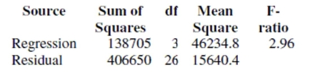
The regression below predicts the daily number of skiers who visit a small ski resort based on three explanatory variables.
The data is a random sample of 30 days from the past two ski seasons. The variables are: SKIERS the number of skiers who visit the resort on that day
SNOW the number of inches of snow on the ground
TEMP the high temperature for the day in degrees .
WEEKDAY an indicator variable, weekday , weekend
Dependent variable is Skiers
squared R squared (adjusted)
with degrees of freedom
 Variable Coefficient SE(Coeff) t-ratio p-value Constant 559.869 76.78 7.29 <0.0001 Snow 1.424 2.70 0.53 0.6019 Temp -1.604 2.77 -0.58 0.5677 Weekend 147.349 51.86 2.84 0.0086
 -Compute a 95% confidence interval for the slope of the variable Weekend, and explain the
meaning of the interval in the context of the problem.
-Compute a 95% confidence interval for the slope of the variable Weekend, and explain the
meaning of the interval in the context of the problem.
The regression below predicts the daily number of skiers who visit a small ski resort based on three explanatory variables.
The data is a random sample of 30 days from the past two ski seasons. The variables are: SKIERS the number of skiers who visit the resort on that day
SNOW the number of inches of snow on the ground
TEMP the high temperature for the day in degrees .
WEEKDAY an indicator variable, weekday , weekend
Dependent variable is Skiers
squared squared (adjusted)
with degrees of freedom
 Variable Coefficient SE(Coeff) t-ratio p-value Constant 559.869 76.78 7.29 <0.0001 Snow 1.424 2.70 0.53 0.6019 Temp -1.604 2.77 -0.58 0.5677 Weekend 147.349 51.86 2.84 0.0086
 -What is the predicted number of skiers for a Saturday with a temperature of 40° F. and a
snow cover of 25 inches?
-What is the predicted number of skiers for a Saturday with a temperature of 40° F. and a
snow cover of 25 inches?
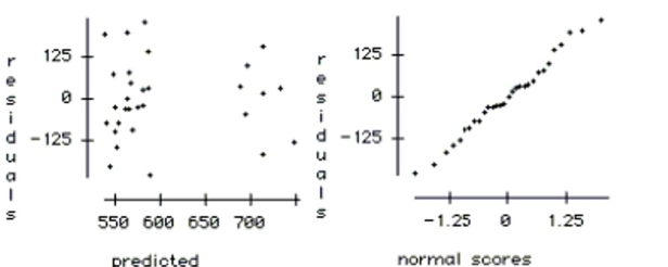
To discourage cheating, a professor makes three different versions of an exam. For the 105
students in her class, she makes 35 copies of each version. The 105 exams are randomly
scrambled, and one copy is given to each student. After the exam, the professor is
concerned that one version might have been easier than the others. She uses a one-way
ANOVA to test whether the average score was different for the three versions. The
ANOVA table and a boxplot of the results are below. Source df Sums of Squares Mean Square F-ratio P-value Version 2 771.943 385.971 4.4317 0.0143 Error 102 8883.49 87.093 Total 104 9655.43
 a. What hypotheses are tested by this ANOVA?
b. Write a sentence describing the conclusion of the test in the context of this problem.
c. Use the plots below to check the ANOVA conditions.
a. What hypotheses are tested by this ANOVA?
b. Write a sentence describing the conclusion of the test in the context of this problem.
c. Use the plots below to check the ANOVA conditions.
Homelessness is a problem in many large U.S. cities. To better understand the problem, a
multiple regression was used to model the rate of homelessness based on several
explanatory variables. The following data were collected for 50 large U.S. cities. The
regression results appear below.  Unemployment percent of residents unemployed
Temperature average yearly temperature (in degrees F.)
Vacancy percent of housing that is unoccupied
Rent Control indicator variable, city has rent control, no rent control
Dependent variable is Homeless
squared squared (adjusted)
with degrees of freedom
Variable Coeff SE(Coeff) t-ratio p-value Constant -4.275 3.465 -1.23 0.2239 Poverty 0.0823 0.0823 1.00 0.3228 Unemployment 0.159 0.218 0.73 0.4699 Temperature 0.135 0.0587 2.30 0.0262 Vacancy -0.247 0.138 -1.79 0.0809 Rent Control 2.944 1.37 2.15 0.0373
a. Using a 5% level of significance, which variables are associated with the number of
homeless in a city?
b. Explain the meaning of the coefficient of temperature in the context of this problem.
c. Explain the meaning of the coefficient of rent control in the context of this problem.
d. Do the results suggest that having rent control laws in a city causes higher levels of
homelessness? Explain.
e. If we created a new model by adding several more explanatory variables, which statistic
should be used to compare them - the R2 or the adjusted R2 ? Explain.
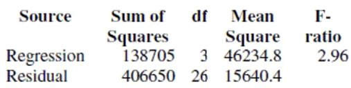
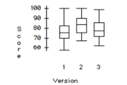
f. Using the plots below, check the regression conditions.
Unemployment percent of residents unemployed
Temperature average yearly temperature (in degrees F.)
Vacancy percent of housing that is unoccupied
Rent Control indicator variable, city has rent control, no rent control
Dependent variable is Homeless
squared squared (adjusted)
with degrees of freedom
Variable Coeff SE(Coeff) t-ratio p-value Constant -4.275 3.465 -1.23 0.2239 Poverty 0.0823 0.0823 1.00 0.3228 Unemployment 0.159 0.218 0.73 0.4699 Temperature 0.135 0.0587 2.30 0.0262 Vacancy -0.247 0.138 -1.79 0.0809 Rent Control 2.944 1.37 2.15 0.0373
a. Using a 5% level of significance, which variables are associated with the number of
homeless in a city?
b. Explain the meaning of the coefficient of temperature in the context of this problem.
c. Explain the meaning of the coefficient of rent control in the context of this problem.
d. Do the results suggest that having rent control laws in a city causes higher levels of
homelessness? Explain.
e. If we created a new model by adding several more explanatory variables, which statistic
should be used to compare them - the R2 or the adjusted R2 ? Explain.
f. Using the plots below, check the regression conditions. 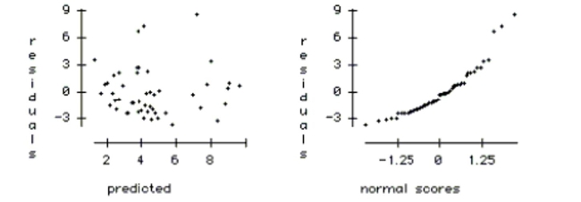
The regression below predicts the daily number of skiers who visit a small ski resort based on three explanatory variables.
The data is a random sample of 30 days from the past two ski seasons. The variables are: SKIERS the number of skiers who visit the resort on that day
SNOW the number of inches of snow on the ground
TEMP the high temperature for the day in degrees .
WEEKDAY an indicator variable, weekday , weekend
Dependent variable is Skiers
R squared squared (adjusted)
with degrees of freedom
 Variable Coefficient SE(Coeff) t-ratio p-value Constant 559.869 76.78 7.29 <0.0001 Snow 1.424 2.70 0.53 0.6019 Temp -1.604 2.77 -0.58 0.5677 Weekend 147.349 51.86 2.84 0.0086
 -If you think that the temperature might affect attendance differently on weekends than on
weekdays, how would you change the regression to test this?
-If you think that the temperature might affect attendance differently on weekends than on
weekdays, how would you change the regression to test this?
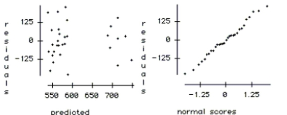
Check the conditions for the regression and comment on whether or not they are satisfied.
Which of the following are NOT characteristics of a good regression model?
Three brands of AAA batteries are compared to see which last longest. Each brand of
battery is tested in four different devices (a TV remote control, a hand-held game, a
miniature flashlight, and a digital camera). The experiment is run once for each
combination of brand and device. The twelve runs are ordered randomly. The time that the
each battery lasts (in minutes) under continuous usage is recorded. Device Brand A Brand B Brand C Remote 1320 1220 1250 Game 480 460 450 Light 245 225 240 Camera 81 72 77
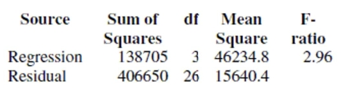
The two-way ANOVA table for response variable Time and factors Brand and Device is
given below. 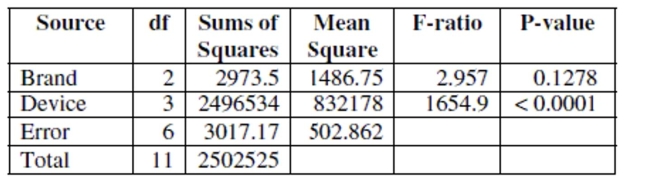 a. Write the model equation for this ANOVA. (Use symbols or words, no numbers.)
b. Test to see whether there is a brand effect. Write the hypotheses being tested, and state
your conclusion using a 5% level of significance. Write your conclusion in the context of
this problem.
c. Explain the role that the device factor plays in this analysis.
d. Can an interaction term be added to this model? Explain.
e. Use the plots below to check the ANOVA conditions.
a. Write the model equation for this ANOVA. (Use symbols or words, no numbers.)
b. Test to see whether there is a brand effect. Write the hypotheses being tested, and state
your conclusion using a 5% level of significance. Write your conclusion in the context of
this problem.
c. Explain the role that the device factor plays in this analysis.
d. Can an interaction term be added to this model? Explain.
e. Use the plots below to check the ANOVA conditions. 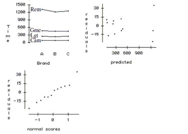
A student wants to build a paper airplane that gets maximum flight distance. She tries
three ways of bending the wing (down, flat, and up) and two levels of nose weight (no and yes
- a paper clip). She randomizes the 12 runs (each condition replicated twice). The analysis
of variance for the 12 runs is shown in the table below along with an interaction plot and
tables of the mean distance for the different wing bends and weights. Source df Sums of Squares Mean Square F-ratio P-value Wing Bend 2 13565.2 6782.58 152.7 <0.0001 Weight 1 6768.75 6768.75 152.39 <0.0001 Interaction 2 186.5 93.25 2.0994 0.2036 Error 6 266.5 44.4167 Total 11 20786.9 Wing Bend Expected Mean Down 145.0 Flat 182.5 Up 227.2 Weight Expected Mean No 161.2 Yes 208.7
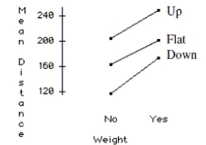 a. Does an additive model seem adequate? Explain.
b. Write a report on this analysis of the data. Include any recommendations you would
give the student on designing the plane.
a. Does an additive model seem adequate? Explain.
b. Write a report on this analysis of the data. Include any recommendations you would
give the student on designing the plane.
The regression below predicts the daily number of skiers who visit a small ski resort based on three explanatory variables.
The data is a random sample of 30 days from the past two ski seasons. The variables are: SKIERS the number of skiers who visit the resort on that day
SNOW the number of inches of snow on the ground
TEMP the high temperature for the day in degrees .
WEEKDAY an indicator variable, weekday , weekend
Dependent variable is Skiers
R squared R squared (adjusted)
with degrees of freedom
 Variable Coefficient SE(Coeff) t-ratio p-value Constant 559.869 76.78 7.29 <0.0001 Snow 1.424 2.70 0.53 0.6019 Temp -1.604 2.77 -0.58 0.5677 Weekend 147.349 51.86 2.84 0.0086
 -Which of the explanatory variables appear to be associated with the number of skiers, and
which do not? Explain how you reached your conclusion.
-Which of the explanatory variables appear to be associated with the number of skiers, and
which do not? Explain how you reached your conclusion.
Here are data about the average January low temperature in cities in the United States, and factors that might allow us to
predict temperature. The data, available for 55 cities, include: 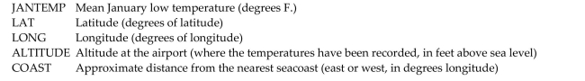 We will attempt to make a regression model to help account for mean January temperature and to understand the effects of
the various predictors.
At each step of the analysis you may assume that things learned earlier in the process are known.
Units Note: The "degrees" of temperature, given here on the Fahrenheit scale, have only coincidental language relationship to
the "degrees" of longitude and latitude. The geographic "degrees" are based on modeling the Earth as a sphere and dividing it
up into 360 degrees for a full circle. Thus 180 degrees of longitude is halfway around the world from Greenwich, England
(0°) and Latitude increases from 0 degrees at the Equator to 90 degrees of (North) latitude at the North Pole.
We will attempt to make a regression model to help account for mean January temperature and to understand the effects of
the various predictors.
At each step of the analysis you may assume that things learned earlier in the process are known.
Units Note: The "degrees" of temperature, given here on the Fahrenheit scale, have only coincidental language relationship to
the "degrees" of longitude and latitude. The geographic "degrees" are based on modeling the Earth as a sphere and dividing it
up into 360 degrees for a full circle. Thus 180 degrees of longitude is halfway around the world from Greenwich, England
(0°) and Latitude increases from 0 degrees at the Equator to 90 degrees of (North) latitude at the North Pole. 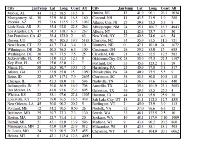 -Now, consider longitude. Should the longitude of a city have an influence on average
January low temperature? Here is the regression: Dependent variable is: JanTemp
R squared R squared (adjusted)
with degrees of freedom
Source Sum of Squares df Mean Square F-ratio Regression 8.34647 1 8.34647 0.045 Residual 9817.18 53 185.230 Variable Coefficient SE(Coeff) t-ratio P-value Intercept 24.0487 11.40 2.11 0.0396 Long 0.026186 0.1234 0.212 0.8327
Test the null hypothesis that the true coefficient of Long is zero in this regression. State the
null and alternative hypotheses and indicate your procedure and conclusion.
-Now, consider longitude. Should the longitude of a city have an influence on average
January low temperature? Here is the regression: Dependent variable is: JanTemp
R squared R squared (adjusted)
with degrees of freedom
Source Sum of Squares df Mean Square F-ratio Regression 8.34647 1 8.34647 0.045 Residual 9817.18 53 185.230 Variable Coefficient SE(Coeff) t-ratio P-value Intercept 24.0487 11.40 2.11 0.0396 Long 0.026186 0.1234 0.212 0.8327
Test the null hypothesis that the true coefficient of Long is zero in this regression. State the
null and alternative hypotheses and indicate your procedure and conclusion.
Of the 23 first year male students at State U. admitted from Jim Thorpe High School, 8 were offered baseball scholarships and
7 were offered football scholarships. The University admissions committee looked at the students' composite ACT scores
(shown in the tabl, wondering if the University was lowering their standards for athletes. Assuming that this group of
students is representative of all admitted students, what do you think?  -Are the two sports teams mean ACT scores different?
Filters
- Essay(0)
- Multiple Choice(0)
- Short Answer(0)
- True False(0)
- Matching(0)